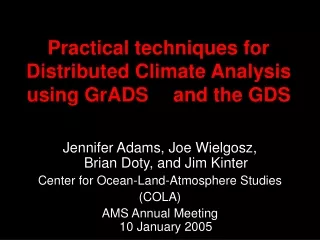
Practical techniques for Distributed Climate Analysis using GrADS and the GDS
290 likes | 305 Vues
Learn about the practical techniques for distributed climate analysis using GrADS and the GDS. This resource covers the features, metadata handling, and examples of analysis techniques.

Practical techniques for Distributed Climate Analysis using GrADS and the GDS
E N D
Presentation Transcript
Practical techniques for Distributed Climate Analysisusing GrADS and the GDS Jennifer Adams, Joe Wielgosz, Brian Doty, and Jim Kinter Center for Ocean-Land-Atmosphere Studies (COLA) AMS Annual Meeting10 January 2005
Outline • Brief description of GrADS and the GDS • New features in upcoming releases • Metadata search engine • Examples of analysis techniques
GrADS is … • Freely available software for the display and analysis of a variety of data types and formats • Gridded and Station (in situ) data • Binary, GRIB , BUFR, NetCDF, HDF-SDS • DODS / OPeNDAP - enabled for accessing distributed data
GrADS Data Server is … • Freely available software that provides access to scientific data for the internet community • Open a URL instead of a local disk file • Data are accessible by a variety of clients: GrADS, Ferret, IDV, IDL, Matlab, ncBrowse, et al. • Any GrADS-readable data may be served • Metadata and data are presented in unified framework • Server-side analysis capability -- Users create data sets that don't yet exist
Outline • Brief description of GrADS and the GDS • New features in upcoming releases • Metadata Handling • Metadata search engine • Examples of analysis techniques
What’s New In GrADS 1.9b4 • Additional metadata may be added to the GrADS descriptor file as attribute comments:@ u String units m/s@ v String units m/s@ lat Float32 minimum -59.875@ lat Float32 maximum 89.875@ global String comment model version 3.2.3 • Attribute comments may appear anywhere in the descriptor file • The 'query attr' command returns all file attributes, distinguishing between those in the descriptor file and those native to the data file (e.g. NetCDF)CAT
What’s New in GDS 1.3 • THREDDS 1.0 catalog • http://cola8.iges.org:9191/dods/thredds • Improved metadata handling • Captures all descriptor file attributes • Allows attribute override • Java-DODS 1.1.7
Outline • Brief description of GrADS and the GDS • New features in upcoming releases • Metadata search engine • How it has been implemented at COLA • Examples of analysis techniques
Basic Components of COLA's Metadata Search Engine • Suite of disk servers -- total disk volume > 15 Tb • Each disk server is running GDS • Disk crawler does nightly search on every disk • Disk crawler finds all viable GrADS descriptor files • Disk crawler writes an XML configuration file for the GDS • Result: Suite of GDSs describes all COLA data sets • Jakarta Lucene search engine indexes each GDS in suite • Search engine uses THREDDS generate the catalog and OPeNDAP to populate all metadata fields • Off-site GDSs are also indexed • Users search using a browser interface or unix command line • Text and numerical searches • Result: A searchable metadata catalog for all of COLA's data
Outline • Brief description of GrADS and the GDS • New features in upcoming releases • Metadata search engine • Examples of analysis techniques • Spatial Averaging • Temporal Averaging & Anomaly Calculation • Intercomparison of data types • Working with Ensembles
Spatial Averaging • Calculate a 50-year time series of monthly global mean 2-meter temperature using NCEP/NCAR Reanalysis data
Script Example server = 'http://cola8.iges.org:9191/dods/' dset = 'rean_2d' lon = '0:0' lat = '0:0'lev = '0:0' time = 'jan1950:jan2000' expr = ' tloop ( aave ( t2m, global ) ) ' 'sdfopen 'server'_expr_{'dset'} {'expr'} {'lon', 'lat', 'lev', 'time'}' 'display result.1'
Temporal Averaging & Anomaly Calculation • Calculate the annual cycle for our 50-year time period • Remove the annual cycle to see the anomaly time series
Script Example server = 'http://cola8.iges.org:9191/dods/' dset = 'rean_2d' lon = '0:0' lat = '0:0'lev = '0:0' time = 'jan1950 : jan2000' expr = ' tloop ( aave ( t2m, global ) ) ' 'sdfopen 'server'_expr_{'dset'} {'expr'} {'lon', 'lat', 'lev', 'time'}' 'display result.1' cache = '_exprcache_7473923027849274839' time = 'jan1950 : dec1950' expr = ' tloop ( ave ( result.1, t+0, t=600, 12 ) ) ' 'sdfopen 'server'_expr_{'cache'} {'expr'} {'lon', 'lat', 'lev', 'time'}' 'set time jan1950 dec1950' 'define annualcycle = result.2' 'modify annualcycle seasonal' 'display result.1-annualcycle'
Synthesis of In-Situ and Gridded Data • GOES Sounder measurements of surface temperature • GOES swath data read into GrADS as station data • 1-hr RUC forecast of 2-meter temperature • GrADS gr2stn function applied to model grid • GrADS oacres function applied to differences at pixel locations
Script Example server1 = 'http://cola8.iges.org:9191/dods'server2 = 'http://nomads.ncdc.noaa.gov:9090/dods' 'open 'server1'/stn/goeseast/sndr/conus/20041224' 'sdfopen 'server2'/NCDC_NOAAPort_RUC/ 200412/20041223/ruc2_236_20041223_2300_fff'' stn = 'ts.1'grid = 'tmp2m.2' 'display 'stn 'display 'grid 'display oacres ( 'grid', gr2stn ( 'grid', 'stn' ) - 'stn' )'
Difference (RUC-GOES) at Pixel LocationsInterpolated to 0.5-degree Grid
NCEP Ensemble Spaghetti Plots • Conventional spaghetti plot illustrates how the forecast model ensemble membersevolve and diverge throughout the forecast period • Animation shows the following: • 500 mb Geopotential Height Analysis (just the 540 dm contour (RED) • 500 mb Geopotential Height Forecast (just the 540 dm contour) from each of 10 ensemble members at 6-hr intervals for a 9-day forecast period (YELLOW ) • Background shading of ensemble mean variance (GRAYSCALE)
A New Spaghetti Recipe • A different kind of spaghetti plot illustrates how the forecast model ensemble members arrived at an agreement as lead time diminished. • Animation shows the following: • 500 mb Geopotential Height Analysis (just the 540 dm contour (RED) • 500 mb Geopotential Height Forecast (just the 540 dm contour) from each of 10 ensemble members at 6-hr intervals BUT each forecast is valid at the analysis time beginning with a 9-day forecast and ending with a 6-hr forecast (YELLOW ) • Background shading of ensemble mean variance (GRAYSCALE)
Summary • GrADS gives you a common interface for gathering and analyzing all kinds of gridded or station data • GrADS Data Server (GDS) provides a unified NetCDF framework for serving a large variety of data sets to the community • Use these tools to enjoy data access and analysis without data management • Open a URL and start working!