Texture
Texture is the spatial arrangement of color/intensities in an image. Explore structural & statistical approaches, edge-based measures, LBP, co-occurrence matrix, Laws’ texture energy features, Gabor filters, and autocorrelation for texture analysis in image processing.

Texture
E N D
Presentation Transcript
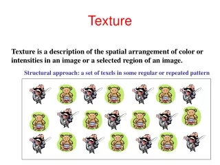
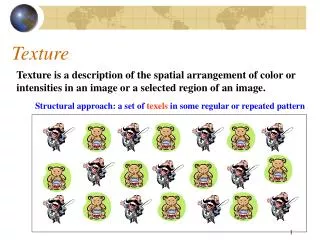
Texture Texture is a description of the spatial arrangement of color or intensities in an image or a selected region of an image. Structural approach: a set of texels in some regular or repeated pattern
Problem with Structural Approach How do you decide what is a texel? Ideas?
Natural Textures from VisTex grass leaves What/Where are the texels?
The Case for Statistical Texture • Segmenting out texels is difficult or impossible in real images. • Numeric quantities or statistics that describe a texture can be • computed from the gray tones (or colors) alone. • This approach is less intuitive, but is computationally efficient. • It can be used for both classification and segmentation.
Some Simple Statistical Texture Measures 1. Edge Density and Direction • Use an edge detector as the first step in texture analysis. • The number of edge pixels in a fixed-size region tells us • how busy that region is. • The directions of the edges also help characterize the texture
Two Edge-based Texture Measures 1. edgeness per unit area 2. edge magnitude and direction histograms Fedgeness = |{ p | gradient_magnitude(p) threshold}| / N where N is the size of the unit area Fmagdir = ( Hmagnitude, Hdirection ) where these are the normalized histograms of gradient magnitudes and gradient directions, respectively.
Example Original Image Frei-Chen Thresholded Edge Image Edge Image
Local Binary Pattern Measure • For each pixel p, create an 8-bit number b1 b2 b3 b4 b5 b6 b7 b8, • where bi = 0 if neighbor i has value less than or equal to p’s • value and 1 otherwise. • Represent the texture in the image (or a region) by the • histogram of these numbers. 1 2 3 100 101 103 40 50 80 50 60 90 4 5 1 1 1 1 1 1 0 0 8 7 6
Example Fids (Flexible Image Database System) is retrieving images similar to the query image using LBP texture as the texture measure and comparing their LBP histograms
Example Low-level measures don’t always find semantically similar images.
Co-occurrence Matrix Features A co-occurrence matrix is a 2D array C in which • Both the rows and columns represent a set of possible • image values. • C (i,j)indicates how many times valueico-occurs with • valuejin a particular spatial relationshipd. • The spatial relationship is specified by a vectord = (dr,dc). d
Co-occurrence Example 1 0 1 2 1 1 0 0 1 1 0 0 0 0 2 2 0 0 2 2 0 0 2 2 0 0 2 2 i j 0 1 2 1 0 3 2 0 2 0 0 1 3 Cd co-occurrence matrix d = (3,1) gray-tone image From Cd we can compute Nd, the normalized co-occurrence matrix, where each value is divided by the sum of all the values.
Co-occurrence Features What do these measure? sums. Energy measures uniformity of the normalized matrix.
But how do you choose d? • This is actually a critical question with all the • statistical texture methods. • Are the “texels” tiny, medium, large, all three …? • Not really a solved problem. Zucker and Terzopoulos suggested using a 2 statistical test to select the value(s) of d that have the most structure for a given class of images.
Laws’ Texture Energy Features • Signal-processing-based algorithms use texture filters • applied to the image to create filtered images from which • texture features are computed. • The Laws Algorithm • Filter the input image using texture filters. • Compute texture energy by summing the absolute • value of filtering results in local neighborhoods • around each pixel. • Combine features to achieve rotational invariance.
Law’s texture masks (2) Creation of 2D Masks E5 L5 E5L5
9D feature vector for pixel • Subtract mean neighborhood intensity from (center) pixel • Apply 16 5x5 masks to get 16 filtered images Fk , k=1 to 16 • Produce 16 texture energy maps using 15x15 windows Ek[r,c] = ∑ |Fk[i,j]| • 9 features defined as follows:
Example: Using Laws Features to Cluster water tiger fence flag grass Is there a neighborhood size problem with Laws? small flowers big flowers
Gabor Filters • Similar approach to Laws • Wavelets at different frequencies and different orientations
Segmentation with Color and Gabor-Filter Texture (Smeulders)
A classical texture measure:Autocorrelation function • Autocorrelation function can detect repetitive patterns of texels • Also defines fineness/coarseness of the texture • Compare the dot product (energy) of non shifted image with a shifted image
Interpreting autocorrelation • Coarse texture function drops off slowly • Fine texture function drops off rapidly • Can drop differently for r and c • Regular textures function will have peaks and valleys; peaks can repeat far away from [0, 0] • Random textures only peak at [0, 0]; breadth of peak gives the size of the texture
Fourier power spectrum • High frequency power fine texture • Concentrated power regularity • Directionality directional texture
Blobworld Texture Features • Choose the best scale instead of using fixed scale(s) • Used successfully in color/texture segmentation in Berkeley’s Blobworld project
Feature Extraction • Input: image • Output: pixel features • Color features • Texture features • Position features • Algorithm: Select an appropriate scale for each pixel and extract features for that pixel at the selected scale feature extraction Pixel Features Polarity Anisotropy Texture contrast Original image
Texture Scale • Texture is a local neighborhood property. • Texture features computed at a wrong scale can lead to confusion. • Texture features should be computed at a scale which is appropriate to the local structure being described. The white rectangles show some sample texture scales from the image.
Scale Selection Terminology • Gradient of the L* component (assuming that the image is in the L*a*b* color space) :▼I • Symmetric Gaussian : Gσ (x, y) = Gσ (x) * Gσ (y) • Second moment matrix: Mσ (x, y)= Gσ (x, y) * (▼I)(▼I)T Ix Iy Ix2 IxIy IxIy Iy2 Notes: Gσ (x, y) is a separable approximation to a Gaussian. σ is the standard deviation of the Gaussian [0, .5, … 3.5]. σ controls the size of the window around each pixel [1 2 5 10 17 26 37 50]. Mσ(x,y) is a 2X2 matrix and is computed at different scales defined by σ.
Scale Selection (continued) • Make use of polarity (a measure of the extent to which the gradient vectors in a certain neighborhood all point in the same direction) to select the scale at which Mσ is computed Edge: polarity is close to 1 for all scales σ Texture: polarity varies with σ Uniform: polarity takes on arbitrary values
Scale Selection (continued) polarity p • n is a unit vector perpendicular to • the dominant orientation. • The notation [x]+ means x if x > 0 else 0 • The notation [x]- means x if x < 0 else 0 • We can think of E+ and E- as measures • of how many gradient vectors in the • window are on the positive side and • how many are on the negative side • of the dominant orientation in the • window. Example: n=[1 1] x = [1 .6] x’ = [-1 -.6]
Scale Selection (continued) • Texture scale selection is based on the derivative of the polarity with respect to scale σ. • Algorithm: • Compute polarity at every pixel in the image for σk = k/2, • (k = 0,1…7). • 2. Convolve each polarity image with a Gaussian with standard • deviation 2k to obtain a smoothed polarity image. • 3. For each pixel, the selected scale is the first value of σ • for which the difference between values of polarity at successive scales is less than 2 percent.
Texture Features Extraction • Extract the texture features at the selected scale • Polarity (polarity at the selected scale) : p = pσ* • Anisotropy: a = 1 – λ2 / λ1 λ1and λ2 denote the eigenvalues of Mσ λ2 /λ1 measures the degree of orientation: when λ1 is large compared to λ2 the local neighborhood possesses a dominant orientation. When they are close, no dominant orientation. When they are small, the local neighborhood is constant. • Local Contrast: C = 2(λ1+λ2)3/2 • A pixel is considered homogeneous if λ1+λ2 < a local threshold
Application to Protein Crystal Images • K-mean clustering result (number of clusters is equal to 10 and similarity measure is Euclidean distance) • Different colors represent different textures Original image in PGM (Portable Gray Map ) format
Application to Protein Crystal Images • K-mean clustering result (number of clusters is equal to 10 and similarity measure is Euclidean distance) • Different colors represent different textures Original image in PGM (Portable Gray Map ) format
References • Chad Carson, Serge Belongie, Hayit Greenspan, and Jitendra Malik. "Blobworld: Image Segmentation Using Expectation-Maximization and Its Application to Image Querying." IEEE Transactions on Pattern Analysis and Machine Intelligence 2002; Vol 24. pp. 1026-38. • W. Forstner, “A Framework for Low Level Feature Extraction,” Proc. European Conf. Computer Vision, pp. 383-394, 1994.

