Download
1 / 25
260 likes | 453 Vues
Texture. Course web page: vision.cis.udel.edu/cv. March 12, 2003 Lecture 12. Announcements . There are some typos in paper linked in HW 2; see course web page for corrections Read Forsyth & Ponce, Chapter 9-9.1, 9.2.2-9.4 on texture for Friday. Outline. Image representations Spatial

E N D
Texture Course web page: vision.cis.udel.edu/cv March 12, 2003 Lecture 12
Announcements • There are some typos in paper linked in HW 2; see course web page for corrections • Read Forsyth & Ponce, Chapter 9-9.1, 9.2.2-9.4 on texture for Friday
Outline • Image representations • Spatial • Frequency • Fourier transform • Definition • Applications
Image Representation • Recall our discussion of basis vectors for coordinate systems: • Describe point as linear combination of ortho-gonal basis vectors: x=a1v1+ ... +anvn • The standard basis for images is the set of unit vectors corresponding to each pixel. A toy example:
Another Image Basis • The standard basis is not the only one we can use to describe an image • E.g., the Hadamard basis (basis images shown here for 2 x 2 images, where black = +1, white = -1) • For the previous example, we can express the image with these new (normalized) basis vectors as: • Coefficients of sum = projection of I onto new basis (dot product) • These are the coordinates of the image in “Hadamard space” • We can also say that I has undergone a Hadamard transform H:
Hadamard Basis for 8 x 8 images Basis images are patterns of rectangular waves with different “frequencies” courtesy of H. Hel-Or Note that the number of basis images = Image dimensions (w x h)
DC component Why Use Another Basis? • The standard basis is convenient, but it yields little insight into the structure of the image • In contrast, consider our example: • The magnitudes of the entries in IH quantify the contribution of each basis image to I • Observation: Dominant textures/edges correspond to higher weights on basis images that look like them • This makes sense, because weights come from dot product, which is correlation • Image compression: Leave out basis images with smallest weights when synthesizing I
Sinusoidal Bases • Binary-valued, rectangular wave pattern of Hadamard basis doesn’t capture real image gradients well • Idea: Use smoothly-varying sinusoidal patterns at different frequencies, angles for basis images
Approximating Arbitrary Functions with Sinusoidal Sums courtesy of H. Hel-Or
Sine & Cosine Functions: Review courtesy of H. Hel-Or
nonlinear operation Sine Function: Amplitude & Phase courtesy of H. Hel-Or
Combining Sine & Cosine Waves for Linear Shifting Observation: Adding a sine wave to a cosine wave with the same frequency yields a scaled and shifted (co)-sine wave with the same frequency courtesy of H. Hel-Or Using this result, we can define a sinusoidal basis
Fourier Basis • The Fourier basis uses the following family of complex sinusoidal functions Real (cos) part (u, v) (1, 0) (1, 1) (0, 5) Imaginary (sin) part
(u, v) r µ Complex Numbers • z = u + iv, where u, v are real and i is imaginary unit equal to • Representations • Cartesian: (u, v) • Polar: reiµ, where r=(u2 + v2)1/2 is called the magnitude, and the phase angle µ=tan-1(v/u) (using Euler formula eix=cosx+isinx) • In Matlab: u = real(z), v = imag(z), r = abs(z), and theta = angle(z)
Fourier Basis Functions: Details • Values are in range [-1, 1] • Frequency: != (u2 + v2)1/2 • Wavelength: ¸= 1/! • Direction: µ = tan-1(v/u) • Minimum ¸of 2 pixels corresponds • to one-pixel wide stripes, so • maximum frequency ! = 1/2 (in • units of inverse pixels—must convert • image dimensions to [-1, 1] range) • These are the highest frequency • basis functions necessary (x, y) = (-1, 1) µ ¸ (1, -1) Basis function for (u, v) = (1, 1)
v Fourier Basis (Imaginary part) Note shift of origin from Hadamard example
Fourier Transform • Given a function f(x, y), its Fourier transform F(u, v) is defined by: • F(u, v) is a complex-valued function • Notation: F(u, v) = F(f(x, y)) • Invertible: F-1(F(u, v)) = f(x, y)
Intuitive Meaning of the Fourier Transform F • Describe image as sum of periodic functions of different frequencies, • Coefficients of terms in sum proportional to prevalence in image of features with corresponding frequencies • Basically, we’re correlating the image with a set of sine-wave patterns whose frequencies and phases are systematically varied. The tabulated results are the Fourier-transformed image • In this sense, we say that F takes an image from the spatial domain to the frequency domain
v Example: Fourier Transform of Image I log(jF(I)j) Phase ofF(I) Note shift of origin (DC component) to center ofF(I). logof magnitude taken because of wide dynamic range
The Fourier Transform in Matlab • Discrete, 2-D Fourier & inverse Fourier transforms are computed by fft2 and ifft2, respectively • fftshift: Move origin (DC component) to image center for display • Example: >> I = imread(‘test.png’); % Load grayscale image >> F = fftshift(fft2(I)); % Shifted transform >> imshow(log(abs(F)),[]); % Show log magnitude >> imshow(angle(F),[]); % Show phase angle
v Example: Fourier Transform of a Fourier Basis-like Function f courtesy of R. Fisher et al. If jF(If)j Biggest weights are on DC component and frequencies corres- ponding to f and -f . Locations tell us the stripe width & angle
v Example: Fourier Transform of another Fourier Basis-like Function f If log(jF(If)j) Thresholded jF(If)j Fourier transform magnitudes ¸ DC peak give us angle here; the additional peaks are harmonics (integer multiples of a frequency). These occur when trying to approximate a square wave
Application: “Unrotating” Text courtesy of R. Fisher et al. Thresholding as before tells us orientation
Fourier Theorem • The convolution of two functions is the same as the product of their Fourier transforms • Given , we have that • Helpful way to convolve efficiently (less so for small kernels) because of: • Fast Fourier Transform (FFT): Algorithm for computing Fourier transform in time nlogn • Method: Apply FFT to “convolvands,” compute product, return IFFT of result—avoids n2 cost