Exploring Stellar Populations Through Mass-Age Pair Simulations and Photometric Analysis
This document discusses a comprehensive approach to studying stellar populations via random simulations of mass-age pairs, synthetic star placement on the Hertzsprung-Russell diagram, and the conversion of stellar parameters. It details the application of photometric errors, crowding evaluations, and the integration of various data points for effective modeling. Emphasis is placed on methodologies such as Blind Fit and tailored fits, which provide insights into star formation histories and the accuracy of stellar evolution models. Lectures from June 2006 provide foundational knowledge and statistical approaches relevant to these studies.

Exploring Stellar Populations Through Mass-Age Pair Simulations and Photometric Analysis
E N D
Presentation Transcript
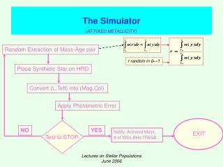
r random in 0↔1 Test to STOP The Simulator (AT FIXED METALLICITY) Random Extraction of Mass-Age pair Place Synthetic Star on HRD Convert (L,Teff) into (Mag,Col) Apply Photometric Error NO YES Notify: Astrated Mass, #of WDs,BHs,TPAGB.. EXIT Lectures on Stellar Populations June 2006
Interpolation between tracks: lifetimes Lectures on Stellar Populations June 2006
Interpolation between Tracks: L and Teff of low mass stars Lectures on Stellar Populations June 2006
Interpolation between Tracks:L and Teff of intermediate mass stars Lectures on Stellar Populations June 2006
Photometric Error: Completeness NGC 1705 (Tosi et al. 2001) Completeness levels: 0.95 % thick 0.75 % thin 0.50 % thick 0.25% thin Lectures on Stellar Populations June 2006
Photometric errors: σDAO and Δm Lectures on Stellar Populations June 2006
Crowding where Sj is the srf density of j stars and σr.e. is the area intercepted # of stars j in one resolution element (r.e.) Probability of j+j blend is Degree of Crowding in the frame With Nr.e resolution elements is depends on SFH: In VII Zw 403 (BCD) we detect with HST 55 RSG, 140 bright AGB and 530 RGT(1) stars/Kpc2 Observed with OmegaCAM we get crow=0.1 at 17,10 and 5.6 Mpc for the 3 kinds resp. In Phoenix (DSp) we detect >4200 RC stars/Kpc2: with OmegaCAM crow is 0.1 already at 2 Mpc Lectures on Stellar Populations June 2006
Another way to put it:(Renzini 1998) # of blends in my frame is # of j stars in my frame (if SSP) is where L is the lum sampled by the r.e. # of blends in my frame becomes # of blends increases with the square of the Luminosity and decreases with the number of resolution elements Lectures on Stellar Populations June 2006
(1) (2) (3) (4) • A.O.: σ(r.e.) ≈ 0.14x0.14 ….. nRGT ≈ 8 in one r.e. • (2) HST: σ(r.e.) ≈ 0.06x0.06…..nRGTxnRGT≈2e-04 … N(r.e.)≈1e+05 • …………………………………………≈ 2e-05….. • (4) GB : σ(r.e.)≈0.3 sq.arcsec….n RGTxnRGT≈0.044…N(r.e.)≈1.3e+04 Pixels and Frames: Example Lectures on Stellar Populations June 2006
How Robust is the Result? The statistical estimator does not account for systematic errors Theoretical Transformed Errors Applied EACH STEP BRINGS ALONG ITS OWN UNCERTAINTIES THE SYSTEMATIC ERROR IS DIFFUCULT TO GAUGE Lectures on Stellar Populations June 2006
Why and How Well does the Method Work? Think of the composite CMD as a superposition of SSPs, each described by an isochrone The number of stars in is proportional to the Mass that went into stars at τ ≈0.1 Gy This is valid for all the PMS boxes, with different proportionality factors Perform the exercise for all isochrones Lectures on Stellar Populations June 2006
Ages: 1112 Gyr [M/H]:-1.75 -1.65 Methods for Solution: Blind Fitused by Hernandez, Gilmore and Valls GabaudHarris and Zaritsky (STARFISH)Cole; Holtzman; Dolphin • Dolphin 2002, MNRAS 332,91: Review of methods and description of Blind fit • Generate a grid of partial model CMD with stars in small ranges of ages and metallicities • Construct Hess diagram for each partial model CMD • Generate a grid of models by combining partial CMDs according to SFR(t) and Z(t) DATA PARTIAL CMD PURE MODEL Lectures on Stellar Populations June 2006
Use a statistical estimator to judge the fit: • mi is the number of synthetic objects in bin i • niis the number of data points in bin i • Minimize fit -- get best fit • + a quantitative measure of the quality of the fit Lectures on Stellar Populations June 2006
My prejudice: • The model CMDs may NOT contain the solution • The method requires a lot of computing: • Does this really improve the solution? • (apart from giving a quantitative estimate • of the quality of the fit) Dolphin: “ The solution with RGB+HB was extremely successful, measuring …the SFH with nearly the same accuracy as the fit to the entire CMD.” If wrong Z is used, the blind method will give a solution, but not THE SOLUTION Lectures on Stellar Populations June 2006
Between 10 and 50 Myr Younger than 10 Myr Between 50 Myr and 1 Gyr Methods for Solution: Tailored Fit Count the stars in the diagnostic boxes: Their number scales with the mass in Stars in the corresponding age range Construct partial CMD constrained to reproduce the star’s counts within the boxes. The partial CMDs are coherently populated also with stars outside the boxes Lectures on Stellar Populations June 2006
Use your knowledge of Stellar evolution to improve the fit AND decide where you cannot improve, and where you need a perfect match • Compare the total simulation to the data The two methods should be viewed as complementary Lectures on Stellar Populations June 2006
Simulation Lectures on Stellar Populations June 2006
What have we learnt When computing the simulations we should pay attention to • The description of the details in the shape of the tracks, and the evolutionary lifetimes(use normalized independent variable) • The description of photometric errors, blending and completeness (evaluate crowding conditions: if there ismore than 1 star per resolution element the photometry is bad; crowding condition depends on sampled luminosity, size of the resolution element and star’s magnitude) Different methods exist to solve for the SFH: the BLIND FIT is statistically good, but does not account for systematic errors; it seems too complicated on one hand, could miss the real target of measuring the mass in stars on the other; the TAILORED FIT goes straight to the point of measuring the mass in stars of the various components of the stellar population; it’s unfit for automatic use; the solution reflects the prejudice of the modeler; the quality of the fit is judged only in a rough way. Lectures on Stellar Populations June 2006