Continuity in Mathematics
440 likes | 489 Vues
Learn about continuity at a point, on open and closed intervals, one-sided limits, and the Intermediate Value Theorem. See examples and definitions to grasp the concept of continuity effectively.

Continuity in Mathematics
E N D
Presentation Transcript
MATH 1910 Chapter 1 Section 4 Continuity and One-Sided Limits
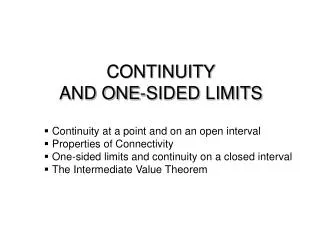
Objectives • Determine continuity at a point and continuity on an open interval. • Determine one-sided limits and continuity on a closed interval. • Use properties of continuity. • Understand and use the Intermediate Value Theorem.
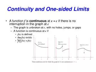
Continuity at a Point and on an Open Interval In mathematics, the term continuous has much the same meaning as it has in everyday usage. Informally, to say that a function f is continuous at x = c means that there is no interruption in the graph of f at c. That is, its graph is unbroken at c and there are no holes, jumps, or gaps.
Continuity at a Point and on an Open Interval Figure 1.25 identifies three values of x at which the graph of f is not continuous. At all other points in the interval (a, b), the graph of f is uninterrupted and continuous. Figure 1.25
Continuity at a Point and on an Open Interval In Figure 1.25, it appears that continuity at x = c can be destroyed by any one of the following conditions. 1. The function is not defined at x = c. 2. The limit of f(x) does not exist at x = c. 3. The limit of f(x) exists at x = c, but it is not equal to f(c). If none of the three conditions above is true, the function f is called continuous at c,as indicated in the following important definition.
Continuity at a Point and on an Open Interval Consider an open interval I that contains a real number c. If a function f is defined on I (except possibly at c), and f is not continuous at c, then f is said to have a discontinuity at c. Discontinuities fall into two categories: removable and nonremovable. A discontinuity at c is called removable if f can be made continuous by appropriately defining (or redefining f(c)).
Figure 1.26 Continuity at a Point and on an Open Interval For instance, the functions shown in Figures 1.26(a) and (c) have removable discontinuities at c and the function shown in Figure 1.26(b) has a nonremovable discontinuity at c.
Example 1 – Continuity of a Function Discuss the continuity of each function.
Example 1(a) – Solution The domain of f is all nonzero real numbers. From Theorem 1.3, you can conclude that f is continuous at every x-value in its domain. At x =0, f has a nonremovable discontinuity, as shown in Figure 1.27(a). In other words, there is no way to define f(0) so as to make the function continuous at x = 0. Figure 1.27(a)
Example 1(b) – Solution cont’d The domain of g is all real numbers except x = 1. From Theorem 1.3, you can conclude that g is continuous at every x-value in its domain. At x = 1, the function has a removable discontinuity, as shown in Figure 1.27(b). If g(1) is defined as 2, the “newly defined” function is continuous for all real numbers. Figure 1.27(b)
Example 1(c) – Solution cont’d The domain of h is all real numbers. The function h is continuous on and , and, because , h is continuous on the entire real line, as shown in Figure 1.27(c). Figure 1.27(c)
Example 1(d) – Solution cont’d The domain of y is all real numbers. From Theorem 1.6, you can conclude that the function is continuous on its entire domain, , as shown in Figure 1.27(d). Figure 1.27(d)
One-Sided Limits and Continuity on a Closed Interval To understand continuity on a closed interval, you first need to look at a different type of limit called a one-sided limit. For example, the limit from the right (or right-hand limit) means that x approaches c from values greater than c [see Figure 1.28(a)]. This limit is denoted as Figure 1.28(a)
One-Sided Limits and Continuity on a Closed Interval Similarly, the limit from the left (or left-hand limit) means that x approaches c from values less than c [see Figure 1.28(b)]. This limit is denoted as Figure 1.28(b)
One-Sided Limits and Continuity on a Closed Interval One-sided limits are useful in taking limits of functions involving radicals. For instance, if n is an even integer,
Example 2 – A One-Sided Limit Find the limit of f(x) = as x approaches –2 from the right. Solution: As shown in Figure 1.29, the limit as x approaches –2 from the right is Figure 1.29
One-Sided Limits and Continuity on a Closed Interval One-sided limits can be used to investigate the behavior of step functions. One common type of step function is the greatest integer function , defined by For instance, and
One-Sided Limits and Continuity on a Closed Interval When the limit from the left is not equal to the limit from the right, the (two-sided) limit does not exist. The next theorem makes this more explicit.
One-Sided Limits and Continuity on a Closed Interval The concept of a one-sided limit allows you to extend the definition of continuity to closed intervals. Basically, a function is continuous on a closed interval when it is continuous in the interior of the interval and exhibits one-sided at the endpoints. This is stated more formally in the next definition. Figure 1.31
One-Sided Limits and Continuity on a Closed Interval Figure 1.31
Example 4 – Continuity on a Closed Interval Discuss the continuity of f(x)= Solution: The domain of f is the closed interval [–1, 1]. At all points in the open interval (–1, 1), the continuity of f follows from Theorems 1.4 and 1.5.
Example 4 – Solution cont’d Moreover, because and you can conclude that f is continuous on the closed interval [–1, 1], as shown in Figure 1.32. Figure 1.32
Properties of Continuity The list below summarizes the functions you have studied so far that are continuous at every point in their domains. By combining Theorem 1.11 with this summary, you can conclude that a wide variety of elementary functions are continuous at every point in their domains.
Example 6 – Applying Properties of Continuity By Theorem 1.11, it follows that each of the functions below is continuous at every point in its domain.
Properties of Continuity The next theorem, which is a consequence of Theorem 1.5, allows you to determine the continuity of composite functions such as
Example 7 – Testing for Continuity Describe the interval(s) on which each function is continuous.
Example 7(a) – Solution The tangent function f(x) = tan x is undefined at At all other points it is continuous.
Example 7(a) – Solution cont’d So, f(x) = tan x is continuous on the open intervals as shown in Figure 1.34(a). Figure 1.34(a)
Example 7(b) – Solution cont’d Because y = 1/x is continuous except at x = 0 and the sine function is continuous for all real values of x, it follows that y = sin (1/x) is continuous at all real values except x = 0. At x = 0, the limit of g(x) does not exist. So, g is continuous on the intervals as shown in Figure 1.34(b). Figure 1.34(b)
Example 7(c) – Solution cont’d This function is similar to the function in part (b) except that the oscillations are damped by the factor x. Using the Squeeze Theorem, you obtain and you can conclude that So, h is continuous on the entire real line, as shown in Figure 1.34(c). Figure 1.34(c)
The Intermediate Value Theorem Theorem 1.3 is an important theorem concerning the behavior of functions that are continuous on a closed interval.
The Intermediate Value Theorem The Intermediate Value Theorem tells you that at least one number c exists, but it does not provide a method for finding c. Such theorems are called existence theorems. A proof of this theorem is based on a property of real numbers called completeness. The Intermediate Value Theorem states that for a continuous function f, if x takes on all values between a and b, f(x)must take on all values between f(a) and f(b).
The Intermediate Value Theorem As an example of the application of the Intermediate Value Theorem, consider a person’s height. A girl is 5 feet tall on her thirteenth birthday and 5 feet 7 inches tall on her fourteenth birthday. Then, for any height h between 5 feet and 5 feet 7 inches, there must have been a time t when her height was exactly h. This seems reasonable because human growth is continuous and a person’s height does not abruptly change from one value to another.
The Intermediate Value Theorem The Intermediate Value Theorem guarantees the existence of at least one number c in the closed interval [a, b] . There may, of course, be more than one number c such that f(c) = k, as shown in Figure 1.35. Figure 1.35
The Intermediate Value Theorem A function that is not continuous does not necessarily exhibit the intermediate value property. For example, the graph of the function shown in Figure 1.36 jumps over the horizontal line given by y =k, and for this function there is no value of c in [a, b] such that f(c) = k. Figure 1.36
The Intermediate Value Theorem The Intermediate Value Theorem often can be used to locate the zeros of a function that is continuous on a closed interval. Specifically, if f is continuous on [a, b] and f(a) and f(b) differ in sign, the Intermediate Value Theorem guarantees the existence of at least one zero of f in the closed interval [a, b] .
Example 8 – An Application of the Intermediate Value Theorem Use the Intermediate Value Theorem to show that the polynomial function has a zero in the interval [0, 1]. Solution: Note that f is continuous on the closed interval [0, 1]. Because it follows that f(0) < 0 and f(1) > 0.
Example 8 – Solution cont’d You can therefore apply the Intermediate Value Theorem to conclude that there must be some c in [0, 1] such that as shown in Figure 1.37. Figure 1.37
The Intermediate Value Theorem The bisection method for approximating the real zeros of a continuous function is similar to the method used in Example 8. If you know that a zero exists in the closed interval [a, b], the zero must lie in the interval [a, (a + b)/2] or [(a + b)/2, b]. From the sign of f([a + b]/2), you can determine which interval contains the zero. By repeatedly bisecting the interval, you can “close in” on the zero of the function.