Face Recognition in Hyperspectral Images

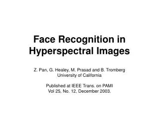
1. Face Recognition in Hyperspectral Images Z. Pan, G. Healey, M. Prasad and B. Tromberg University of California Published at IEEE Trans. on PAMI Vol 25, No. 12, December 2003.

2. Introduction What is a hyperspectral Image? visible electromagnetic spectrum 0.4 0.7 µm Red, RGB Green, Blue Channels

3. Introduction What is a hyperspectral Image? UV = Ultra Violet Vis = VisibleNIR = Near infraredSWIR = Short wavelength infraredMWIR = Medium wavelength infraredLWIR = Long wavelength infrared

4. Introduction “Hyperspectral cameras provide useful discriminants for human face that cannot be obtained by other imaging methods.”

5. Introduction • The utility of using near-infrared (NIR) hyperspectral images for face recognition is studied; • Spectral measurements over the NIR allow sensing subsurface tissue structures; • Subsurface tissue: • Significantly different from person to person, • Relatively stable over time, • Nearly invariant to face orientations and expressions.

6. Introduction “Significantly different from person to person”

7. Introduction “Nearly invariant to face orientations”

8. Data Collection • 200 subjects; • 31 spectral bands (0.7-1.0µm); • Tunable filter; • 468x498 spatial resolution; • Uniform illumination; • 10 seconds each image.

9. Data Collection

10. Data Collection 7 images for each subject and at most 5 regions (17x17) sampled: 20 subjects took part of different imaging sessions:

11. Experiments Setup • Cumulative Match Characteristic (CMC) curves. • Minimum Mahalanobis Distance from query to gallery: where ωxis 1 or 0, if region x was sampled or not; Dx(i, j) is computed from the average intensities of the sampled region x of i and j.

12. First Experiment - Verification of utility of various tissues types for hyperspectral face recognition; - Only frontal images were used (Gallery: fg; Query: fa, fb).

13. First Experiment Better performance is achieved when different tissues are combined

14. First Experiment Changes in expression do not impact significantly the hyperspectral discriminants

15. First Experiment Forehead is the least affected by change of expressions

16. Second Experiment - Examination of the impact of changes in face orientation for hyperspectral face recognition; - Only frontal images were used (Gallery: fg; Query: all others).

17. Second Experiment 45° - 75% for n = 1 and 94% for n = 5; 90° - 80% for n = 10. The distance function assumes that tissue spectral reflectance does not depend on photometric angles.

18. Second Experiment Performance degrades as the size of the subset considered increases.

19. Analysesof First and Second Experiment

20. Analysesof First and Second Experiment

21. Third Experiment • Examination of variance of hyperspectral discriminants over time; • 20 subjects imaged between 3 days and 5 weeks after the first session; • The same 200 subject gallery is used.

22. Third Experiment - Similar results for images from different times; - Significant reduction of performance over “single day” images

23. Third Experiment The difference in performance can be attributed to changes in subject condition: - blood flow; - water concentration; - blood oxygenation; - melanin concentration; Also - sensor characteristics.

24. Questions?

25. Face Recognition on Fitting a 3D Morphable Model V. Blanz and T. Vetter Published at IEEE Trans. on PAMI Vol 25, No. 9, September 2003.

26. Introduction • Color values in a face image do not depend only on the person identity (pose and illumination); • Goal: separate the characteristics of a face (shape and texture) from conditions of image acquisition; • The conditions may be described consistently across the entire image by a small set of extrinsic parameters;

27. Introduction • The algorithm developed combines deformable 3D models with CG simulations of illumination and projection; • It makes face shape and texture fully independent of extrinsic parameters; • Given a single image of a person, the algorithm automatically estimates face 3D shape, texture, and all relevant 3D scene parameters.

28. Model-Based Recognition

29. Morphable Model • Vector space constructed such that any “convex combination” of shape and texture vectors Si and Ti describes a human face; • Continuous changes in model parameters generate a smooth transition that moves the initial surface toward a final one;

30. Database of 3D Laser Scans • Laser scans of 200 faces were used to create the morphable model;

31. Correspondence • Establish dense point-to-point correspondence between each face and a reference face: • Generalization of “Optical Flow” to 3D surfaces is used to determine the vector field: Vi

32. Generalized Optical Flow To find the face vector field, the following expression must be minimized for a neighborhood R (5x5):

33. Face Vectors • One scanned face is chosen as reference I0 • Reference shape and texture vectors are defined from conversion of each cylindrical coordinate to Cartesian coordinates:

34. Face Vectors • For a novel scan I, the flow field from I0 to I is computed and converted to cartesian coordinates (S and T).

35. Principal Component Analysis • PCA is performed on Si and Ti • Shape and texture eigenvectors (si and ti) and variances (σS and σT) are computed:

36. Model Fitting • Given a novel face image, the parameters and are found to provide the reconstruction of the 3D shape; • Pose, camera focal length, light intensity, color and direction are automatically found;

37. Model Fitting

38. Model Fitting • Optimization of shape coefficients and texture coefficients , along with pose angles, translation and focal length parameters, Lambertian light intensity and direction, contrast, and gains and offsets of color channels (ρ); • Cost Function: • Optimization method: Stochastic Newton Algorithm. • Similar to stochastic gradient descent algorithm; • Makes use of first derivative of E;

39. Experiments • Model fitting and identification were tested on PIE (4488 images) and FERET (1940 images) databases; • None of the faces are in the model database; • Feature points manually defined: • Gallery and Query recognition approach.

40. Results of Model Fitting

41. Results of Model Fitting

42. Results of Recognition • Metrics used for comparison: • Sum of Mahalanobis Distances dM = ||c1-c2||^2 • Cosine of the angle between two vectors dA=<c1,c2>/||c1||.||c2|| • Maximum-Likelihood and LDA • c is a face, represented by shape and texture coefficients; dW is superior because it takes into account fitting inaccuracy (different coefficients for the same subject)

43. Results of Recognition

44. Results of Recognition

45. Results of Recognition

46. Comment • Fitting process depends on user interaction and takes 4.5 minutes on a Pentium 3 2GHz.

47. Questions?