Direct Measurement of Capillary Cortical Blood Volume Using Multiphoton Laser Scanning Microscopy
This study presents a novel approach for in vivo measurement of capillary blood volume in the cortex of anesthetized mice, utilizing two-photon laser scanning microscopy. By injecting fluorescent dyes intravascularly, a detailed imaging of blood vessels is achieved, capturing depths up to 600 µm below the dura. The method demonstrates high spatial and temporal resolutions while allowing for rapid acquisition and analysis, revealing significant variability in capillary blood volume (CBV) among subjects under various physiological conditions. Detailed image processing techniques are employed to enhance data accuracy.

Direct Measurement of Capillary Cortical Blood Volume Using Multiphoton Laser Scanning Microscopy
E N D
Presentation Transcript
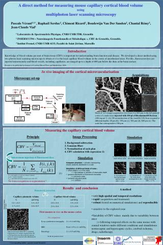
a. Slice of the original stack without noise b. Same slice as (a) after noises simulation c. Same slice after image processing f. Z-projection of the noisy stack after image processing CBV = 1,7 % e. Z-projection of the noisy stack (corresponds to (b)) d. Z-projection of the original stack without noise CBV = 1,6 % In vivo imaging of the cortical microvascularisation Acquisitions Microscopy set-up b c Scanning mirrors (x,y) FemtosecondlaserTi sa d e Intensityvariator Dichroïcmirror λ780 nm red FilterCube a green Stack of 121 images acquired in vivo from 0 to 600 µm in the left parietal cortex of a nude mice injected with 100 µl of Rhodamine6B Dextran (100 mg.ml-1) (A) 3D reconstruction of the stack B,C,D) Scan acquired at different depths :40 µm (b), 150 µm (c), 300 µm (d), 600 µm (e). The scale bar corresponds to 100 µm ExternalPMTs 20x NA 0.95 BioradInterface mouse Results and conclusion • A method • with high spatial and temporal resolutions • rapid (acquisition and treatment) • robust (tested on numerical simulations) and reproducible • sensitive to the explored zone • Variability of CBV values mainly due to variability between mice following temporal effects on the same mouse with cranial windows under different conditions and stimulations: normocapnic and hypercapnic cycles, cerebral ischemia, drugs, radiotherapy. Hematocrit correction Extremal Valueson 7 mice First mesure in vivo on the mouse cortex For normalization For comparison 100 µm Typical stack from which CBV is estimated.Z-projection of 51 images acquired from 100 to 200 µm below the dura in the left parietal cortex of a mouse injected with a Rhodamin BDextran solution In the rat parietal cortex A direct method for measuring mouse capillary cortical blood volume using multiphoton laser scanning microscopy Pascale Vérant1,3,*, Raphaël Serduc2, Clément Ricard2, Boudewijn Van Der Sanden2, Chantal Rémy2, Jean-Claude Vial1 1 Laboratoire de Spectrométrie Physique, CNRS UMR 5588, Grenoble 2 INSERM U594 « Neuroimagerie Fonctionnelle et Métabolique », CHU de Grenoble, Grenoble. 3 Institut Fresnel, CNRS UMR 6133, Faculté de Saint Jérôme, Marseille Introduction Knowledge of blood volume per unit of brain tissue (CBV) is important for understanding brain function and disease. We developed a direct method using two-photon laser scanning microscopy to obtain in vivo the local capillary blood volume in the cortex of anesthetized mice. For this, fluorescent dyes are injected intravenously and blood vessels, including capillaries, are imaged up to a depth of 600 µm below the dura at the brain surface. Results to be published in Journal of Cerebral Blood Flow and Metabolism 2006. Measuring the capillary cortical blood volume Principle Image Processing Simulation • Background subtraction • Gaussian Blurr • Normalization of each plan • CBV calculation with expression (1) Intravenous injection of fluorescent dyes Simulation • Computer phantom = cylinders representing vessels randomly distributed in a cube • Simulation of different kinds of noise : • offset added in ¼ of the stack > dye leakage or variation of observation depth • gaussian distribution of fluorescent intensities <=>photonic noise • randomly saturated pixels <=> artifacts (1) N = total number of voxels in volume of interest. (i,j,k) = voxels’s identifier. Imax = maximum intensity per plan k (gray value 255). No form recognition or segmentation ! * Corresponding author : pascale.verant@fresnel.fr