Search Algorithm Lecture-14
This lecture explores various algorithms for implementing SELECT and JOIN operations in databases. It covers search methods for simple and complex selections, including linear search, binary search, primary and secondary indexing, and the use of clustering indexes. Additionally, it explains conjunctive selection techniques and different methods for implementing joins such as nested-loop and single-loop joins. The optimization of query execution based on existing access paths is emphasized to minimize data retrieval time and improve overall efficiency.


Search Algorithm Lecture-14
E N D
Presentation Transcript
Algorithms for SELECT and JOIN Operations Implementing the SELECT Operation : Search Methods for Simple Selection: • S1. Linear search (brute force): Retrieve every record in the file, and test whether its attribute values satisfy the selection condition. • S2. Binary search: If the selection condition involves an equality comparison on a key attribute on which the file is ordered, binary search (which is more efficient than linear search) can be used. • S3. Using a primary index or hash key to retrieve a single record: If the selection condition involves an equality comparison on a key attribute with a primary index (or a hash key), use the primary index (or the hash key) to retrieve the record.
Algorithms for SELECT and JOIN Operations Implementing the SELECT Operation (cont.): Search Methods for Simple Selection: • S4. Using a primary index to retrieve multiple records: If the comparison condition is >, ≥, <, or ≤ on a key field with a primary index, use the index to find the record satisfying the corresponding equality condition, then retrieve all subsequent records in the (ordered) file. • S5. Using a clustering index to retrieve multiple records: If the selection condition involves an equality comparison on a non-key attribute with a clustering index, use the clustering index to retrieve all the records satisfying the selection condition. • S6. Using a secondary (B+-tree) index: On an equality comparison, this search method can be used to retrieve a single record if the indexing field has unique values (is a key) or to retrieve multiple records if the indexing field is not a key. In addition, it can be used to retrieve records on conditions involving >,>=, <, or <=. (FOR RANGE QUERIES)
Algorithms for SELECT and JOIN Operations Implementing the SELECT Operation (cont.): Search Methods for Complex Selection: • S7. Conjunctive selection: If an attribute involved in any single simple condition in the conjunctive condition has an access path that permits the use of one of the methods S2 to S6, use that condition to retrieve the records and then check whether each retrieved record satisfies the remaining simple conditions in the conjunctive condition. • S8. Conjunctive selection using a composite index: If two or more attributes are involved in equality conditions in the conjunctive condition and a composite index (or hash structure) exists on the combined field, we can use the index directly.
Algorithms for SELECT and JOIN Operations Implementing the SELECT Operation (cont.): Search Methods for Complex Selection: • S9. Conjunctive selection by intersection of record pointers: This method is possible if secondary indexes are available on all (or some of) the fields involved in equality comparison conditions in the conjunctive condition and if the indexes include record pointers (rather than block pointers). Each index can be used to retrieve the record pointers that satisfy the individual condition. The intersection of these sets of record pointers gives the record pointers that satisfy the conjunctive condition, which are then used to retrieve those records directly. If only some of the conditions have secondary indexes, each retrieved record is further tested to determine whether it satisfies the remaining conditions.
Algorithms for SELECT and JOIN Operations (7) Implementing the SELECT Operation (cont.): • Whenever a single condition specifies the selection, we can only check whether an access path exists on the attribute involved in that condition. If an access path exists, the method corresponding to that access path is used; otherwise, the “brute force” linear search approach of method S1 is used. • For conjunctive selection conditions, whenever more than one of the attributes involved in the conditions have an access path, query optimization should be done to choose the access path that retrieves the fewest records in the most efficient way .
Algorithms for SELECT and JOIN Operations (8) Implementing the JOIN Operation: • Join (EQUIJOIN, NATURAL JOIN) • two–way join: a join on two files e.g. R A=B S • multi-way joins: joins involving more than two files. e.g. R A=B S C=D T • Examples (OP6): EMPLOYEE DNO=DNUMBER DEPARTMENT (OP7): DEPARTMENT MGRSSN=SSN EMPLOYEE
Algorithms for SELECT and JOIN Operations (9) Implementing the JOIN Operation (cont.): Methods for implementing joins: • J1. Nested-loop join (brute force): For each record t in R (outer loop), retrieve every record s from S (inner loop) and test whether the two records satisfy the join condition t[A] = s[B]. • J2. Single-loop join (Using an access structure to retrieve the matching records): If an index (or hash key) exists for one of the two join attributes — say, B of S — retrieve each record t in R, one at a time, and then use the access structure to retrieve directly all matching records s from S that satisfy s[B] = t[A].
Algorithms for SELECT and JOIN Operations (10) Implementing the JOIN Operation (cont.): Methods for implementing joins: • J3. Sort-merge join: If the records of R and S are physically sorted (ordered) by value of the join attributes A and B, respectively, we can implement the join in the most efficient way possible. Both files are scanned in order of the join attributes, matching the records that have the same values for A and B. In this method, the records of each file are scanned only once each for matching with the other file—unless both A and B are non-key attributes, in which case the method needs to be modified slightly.
Algorithms for SELECT and JOIN Operations (11) Implementing the JOIN Operation (cont.): Methods for implementing joins: • J4. Hash-join: The records of files R and S are both hashed to the same hash file, using the same hashing function on the join attributes A of R and B of S as hash keys. A single pass through the file with fewer records (say, R) hashes its records to the hash file buckets. A single pass through the other file (S) then hashes each of its records to the appropriate bucket, where the record is combined with all matching records from R.
B-TREE • A B-tree is a specialized multiway tree designed especially for use on disk • In a B-tree each node may contain a large number of keys • Only a small number of nodes must be read from disk to retrieve an item • The goal is to get fast access to the data
B-TREE • A multiway tree of order m is an ordered tree where each node has at most m children. For each node, if k is the actual number of children in the node, then k - 1 is the number of keys in the node. If the keys and subtrees are arranged in the fashion of a search tree, then this is called a multiway search tree of order m. For example, the following is a multiway search tree of order 4. Note that the first row in each node shows the keys, while the second row shows the pointers to the child nodes. • Of course, in any useful application there would be a record of data associated with each key, so that the first row in each node might be an array of records where each record contains a key and its associated data. Another approach would be to have the first row of each node contain an array of records where each record contains a key and a record number for the associated data record, which is found in another file. This last method is often used when the data records are large.
Hash tables • hash table: an array of some fixed size, that positions elements according to an algorithm called a hash function hash func. h(element) length –1 elements (e.g., strings) hash table
Hashing, hash functions • The idea: somehow we map every element into some index in the array ("hash" it);this is its one and only place that it should go • Lookup becomes constant-time: simply look at that one slot again later to see if the element is there • add, remove, contains all become O(1) ! • For now, let's look at integers (int) • a "hash function" h for int is trivial: store int i at index i (a direct mapping) • if i >= array.length, store i at index(i % array.length) • h(i) = i % array.length
Hash function in action • Add these elements to thehash table: • 89 • 18 • 49 • 58 • 9
Hash function example • elements = Integers • h(i) = i % 10 • add 41, 34, 7, and 18 • constant-time lookup: • just look at i % 10 again later • We lose all ordering information: • getMin, getMax, removeMin, removeMax • the various ordered traversals • printing items in sorted order
Hash collisions • collision: the event that two hash table elements map into the same slot in the array • example: add 41, 34, 7, 18, then 21 • 21 hashes into the same slot as 41! • 21 should not replace 41 in the hash table;they should both be there collision resolution: means for fixing collisions in a hash table
Linear probing • linear probing: resolving collisions in slot i by putting the colliding element into the next available slot (i+1, i+2, ...) • add 41, 34, 7, 18, then 21, then 57 • 21 collides (41 is already there), so we search ahead until we find empty slot 2 • 57 collides (7 is already there), so we search ahead twice until we find empty slot 9 • lookup algorithm becomes slightly modified; we have to loop now until we find the element or an empty slot • what happens when the table gets mostly full?
Clustering problem • clustering: nodes being placed close together by probing, which degrades hash table's performance • add 89, 18, 49, 58, 9 • now searching for the value 28 will have to check half the hash table! no longer constant time...
Quadratic probing • quadratic probing: resolving collisions on slot i by putting the colliding element into slot i+1, i+4, i+9, i+16, ... • add 89, 18, 49, 58, 9 • 49 collides (89 is already there), so we search ahead by +1 to empty slot 0 • 58 collides (18 is already there), so we search ahead by +1 to occupied slot 9, then +4 to empty slot 2 • 9 collides (89 is already there), so we search ahead by +1 to occupied slot 0, then +4 to empty slot 3 • clustering is reduced • what is the lookup algorithm?
Chaining • chaining: All keys that map to the same hash value are kept in a linked list 10 22 12 42 107
Load factor • load factor: ratio of elements to capacity • load factor = size / capacity = 6 / 10 = 0.6
Rehashing, hash table size • rehash: increasing the size of a hash table's array, and re-storing all of the items into the array using the hash function • can we just copy the old contents to the larger array? • When should we rehash? Some options: • when load reaches a certain level (e.g., = 0.5) • when an insertion fails • What is the cost (Big-Oh) of rehashing? • what is a good hash table array size? • how much bigger should a hash table get when it grows?
Hash table removal • lazy removal: instead of actually removing elements, replace them with a special REMOVED value • avoids expensive re-shuffling of elements on remove • example: remove 18 --> • lookup algorithm becomes slightly modified • what should we do when we hit a slot containing the REMOVED value? • keep going • add algorithm becomes slightly modified • what should we do when we hit a slot containing the REMOVED value? • use that slot, replace REMOVED with the new value • add(17) --> slot 8
Hashing practice problem • Draw a diagram of the state of a hash table of size 10, initially empty, after adding the following elements:7, 84, 31, 57, 44, 19, 27, 14, and 64Assume that the hash table uses linear probing.Assume that rehashing occurs at the start of an add where the load factor is 0.75. • Repeat the above problem using quadratic probing.
Writing a hash function • If we write a hash table that can store objects, we need a hash function for the objects, so that we know what index to store them We want a hash function to: • be simple/fast to compute • map equal elements to the same index • map different elements to different indexes • have keys distributed evenly among indexes
Hash function for strings • elements = Strings • let's view a string by its letters: • String s : s0, s1, s2, …, sn-1 • how do we map a string into an integer index?(how do we "hash" it?) • one possible hash function: • treat first character as an int, and hash on that • h(s) = s0 % array.length • is this a good hash function? When will strings collide?
Better string hash functions • view a string by its letters: • String s : s0, s1, s2, …, sn-1 • another possible hash function: • treat each character as an int, sum them, and hash on that • h(s) = % array.length • what's wrong with this hash function? When will strings collide? • a third option: • perform a weighted sum of the letters, and hash on that • h(s) = % array.length
Analysis of hash table search • load: the load of a hash table is the ratio: no. of elements array size • analysis of search, with linear probing: • unsuccessful: • successful:
Analysis of hash table search • analysis of search, with chaining: • unsuccessful: (the average length of a list at hash(i)) • successful: 1 + (/2)(one node, plus half the avg. length of a list (not including the item))
Compound collections • Collections can be nested to represent more complex data • example: A person can have one or many phone numbers • want to be able to quickly find all of a person's phone numbers, given their name • implement this example as a HashMap of Lists • keys are Strings (names) • values are Lists (e.g ArrayList) of Strings, where each String is one phone number String List<String> name --> list of phone numbers "Phil" --> ["234-8793", "439-8575", ...]
Performance tuning • Performance tuning is the main activity associated with performance management. • Reduced to its most basic level, tuning consists of finding and eliminating bottlenecks — a condition that occurs, and is revealed, when a piece of hardware or software in a server approaches the limits of its capacity.
The Tuning Cycle • The tuning cycle, which is an iterative series of controlled performance experiments.. • Repeat the four phases of the tuning cycle shown below until you achieve the performance goals that you established prior to starting the tuning process. • Tuning Cycle:
Tuning Cycle • Collecting The Collecting phase is the starting point of any tuning exercise. Gathering data with the collection of performance counters that are chosen for a specific part of the system. • Analyzing After you have collected the performance data that you require for tuning the selected part of the system, you need to analyze the data to determine bottlenecks.
Tuning Cycle • Configuring After you have collected your data and completed the analysis of the results, you can determine which part of the system is the best candidate for a configuration change and implement this change. • Testing After implementing a configuration change, you must complete the appropriate level of testing to determine the impact of the change on the system that you are tuning.
Tuning Cycle • When testing, be sure to: • Check the correctness and performance of the application that you are using for testing by looking for memory leaks and inordinate delays in response to client requests. • Ensure that all tests are working correctly. • Make sure you can repeat all tests by using the same transaction mix and the same clients generating the same load. • Document changes and results.
Database Performance Tuning • DBMS Installation • Setting installation parameters • Memory Usage • Set cache levels • Choose background processes • Input / Output (I/O) Contention • Distribution of heavily accessed files • CPU Usage • Monitor CPU load • Application tuning • Modification of SQL code in applications