Download
1 / 49
510 likes | 987 Vues
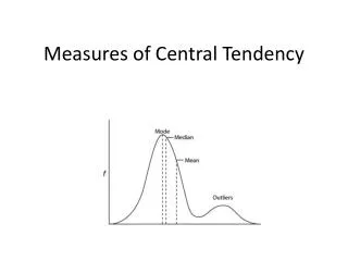
Measures of Central Tendency. By Rahul Jain. The Motivation. Measure of central tendency are used to describe the typical member of a population. Depending on the type of data, typical could have a variety of “best” meanings. We will discuss four of these possible choices.

E N D
Measures of Central Tendency By Rahul Jain
The Motivation • Measure of central tendency are used to describe the typical member of a population. • Depending on the type of data, typical could have a variety of “best” meanings. • We will discuss four of these possible choices.
4 Measures of Central Tendency • Mean – the arithmetic average. This is used for continuous data. • Median – a value that splits the data into two halves, that is, one half of the data is smaller than that number, the other half larger. May be used for continuous or ordinal data. • Mode – this is the category that has the most data. As the description implies it is used for categorical data. • Midrange – not used as often as the other three, it is found by taking the average of the lowest and highest number in the data set. Also primarily used for continuous data.
Measures of Central Tendency • The central tendency is measured by averages. These describe the point about which the various observed values cluster. • In mathematics, an average, or central tendency of a data set refers to a measure of the "middle" or "expected" value of the data set.
Mean • To find the mean, add all of the values, then divide by the number of values. • The lower case, Greek letter mu is used for population mean. • An “x” with a bar over it, read x-bar, is used for sample mean.
Arithmetic Mean of Group Data • if are the mid-values and are the corresponding frequencies, where the subscript ‘k’ stands for the number of classes, then the mean is
Median • The median is a number chosen so that half of the values in the data set are smaller than that number, and the other half are larger. • To find the median • List the numbers in ascending order • If there is a number in the middle (odd number of values) that is the median • If there is not a middle number (even number of values) take the two in the middle, their average is the median
Median • The implication of this definition is that a median is the middle value of the observations such that the number of observations above it is equal to the number of observations below it. If “n” is Even If “n” is odd
Median of Group Data • L0 = Lower class boundary of the median class • h = Width of the median class • f0 = Frequency of the median class • F = Cumulative frequency of the pre- median class
Steps to find Median of group data • Compute the less than type cumulative frequencies. • Determine N/2 , one-half of the total number of cases. • Locate the median class for which the cumulative frequency is more than N/2 . • Determine the lower limit of the median class. This is L0. • Sum the frequencies of all classes prior to the median class. This is F. • Determine the frequency of the median class. This is f0. • Determine the class width of the median class. This is h.
Mode • The mode is simply the category or value which occurs the most in a data set. • If a category has radically more than the others, it is a mode. • Generally speaking we do not consider more than two modes in a data set. • No clear guideline exists for deciding how many more entries a category must have than the others to constitute a mode.
Obvious Example • There is obviously more yellow than red or blue. • Yellow is the mode. • The mode is the class, not the frequency.
No Mode Category Frequency 1 51 2 51 3 66 4 62 5 65 6 57 7 47 8 43 • 64 • Although the third category is the largest, it is not sufficiently different to be called the mode.
Example-2: Find Mean, Median and Mode of Ungroup Data The weekly pocket money for 9 first year pupils was found to be: 3 , 12 , 4 , 6 , 1 , 4 , 2 , 5 , 8 Mean 5 Median 4 Mode 4
Mode of Group Data • L1 = Lower boundary of modal class • Δ1 = difference of frequency between modal class and class before it • Δ2 = difference of frequency between modal class and class after • H = class interval
Steps of Finding Mode • Find the modal class which has highest frequency • L0 = Lower class boundary of modal class • h = Interval of modal class • Δ1 = difference of frequency of modal class and class before modal class • Δ2 = difference of frequency of modal class and class after modal class
Midrange • The midrange is the average of the lowest and highest value in the data set. • This measure is not often used since it is based strictly on the two extreme values in the data.
Measures of Variation Same mean, but y varies more than x.
Three Measures of Variation • While there are other measures, we will look at only three: • Variance • Standard deviation • Coefficient of variation • Population mean and sample mean use an identical formula for calculation. • There is a minor difference in the formulas for variation.
Population Variance • The population variance, σ2, is found using either of the formulas to the right. • The differences are squared to prevent the sum from being zero for all cases. • N is the size of the population, μ is the population mean. • Note that variance is always positive if x can take on more than one value.
Population Standard Deviation • The standard deviation can be thought of as the average amount we could expect the x’s in the population to differ from the mean value of the population. • To get the standard deviation, simply take the square root of the variance.
Sample Variance • The sample variance, s2, is found using either of the formulas to the right. • The differences are squared to prevent the sum from being zero for all cases. • The sample size is n, x-bar is the sample mean. • Note that n-1 is used rather than n. This adjustment prevents bias in the estimate.
Sample Standard Deviation • Just like the standard deviation of a population, to find the standard deviation of a sample, take the square root of the sample variance.
Coefficient of Variation • The measures discussed so far are primarily useful when comparing members from the same population, or comparing similar populations. • When looking at two or more dissimilar populations, it doesn’t make any more sense to compare standard deviations than it does to compare means.
Coefficient of Variation Cont. • Example 1: Weight loss programs A and B. • Two different programs with the same goal and target population. • While program B averages more weight loss, it also has less consistent results.
Coefficient of Variation Cont. • Example 2: Weight loss program A and tax refund B. • Two different programs with different goals and different target populations. • We know that average weight loss and average tax refund are not comparable. Are the standard deviations comparable?
Coefficient of Variation Cont. • In the last example we can see an argument that standard deviation does not give the complete picture. • The coefficient of variation addresses this issue by establishing a ratio of the standard deviation to the mean. This ratio is expressed as a percentage.
Coefficient of Variation Cont. • Looking at the two examples. We see that in both cases the standard deviation for B is twice that of A. • In the first example we have almost twice the relative variation in B. • In the second example, we have a little over 16 times as much variation in A.
Measures of Position The dot on the left is at about -1, the dot on the right is at approximately 0.8. But where are they relative to the rest of the values in this distribution.
Quartiles, Percentiles and Other Fractiles • We will only consider the quartile, but the same concept is often extended to percentages or other fractions. • The median is a good starting point for finding the quartiles. • Recall that to find the median, we wanted to locate a point so that half of the data was smaller, and the other half larger than that point.
Quartile • For quartiles, we want to divide our data into 4 equal pieces. Suppose we had the following data set (already in order) 2 3 7 8 8 8 9 13 17 20 21 21 Choosing the numbers 7.5, 8.5, and 18.5 as markers would Divide the data into 4 groups, each with three elements. These numbers would be the three quartiles for this data set.
Quartiles Continued • Conceptually, this is easy, simply find the median, then treat the left hand side as if it were a data set, and find its median; then do the same to the right hand side. • This is not always simple. Consider the following data set. • 3 3 3 3 3 5 6 8 8 8 8 8 9 • The first difficulty is that the data set does not divide nicely. • Using the rules for finding a median, we would get quartiles of 3, 6 and 8. • The second difficulty is how many of the 3’s are in the first quartile, and how many in the second?
Quartiles Continued • For this course, let’s pretend that this is not an issue. • I will give you the quartiles. • I will not ask how many are in a quartile.
Interquartile Range • One method for identifying these outliers, involves the use of quartiles. • The interquartile range (IQR) is Q3 – Q1. • All numbers less than Q1 – 1.5(IQR) are probably too small. • All numbers greater than Q3 + 1.5(IQR) are probably too large.
Measures of Variation: Variance & Standard Deviationfor GROUPED DATA • The grouped variance is • The grouped standard deviation is
Example 3-24 (p130): Miles Run per Week Find the variance and the standard deviation for the frequency distribution below. The data represents the number of miles that 20 runners ran during one week. 8 13 18 23 28 33 38 1·8 = 8 2·13 = 26 3·18 = 54 5·23 = 115 4·28 =108 3·33 = 99 2·38 = 76 Σf·Xm= 486 1(8-24.3)2 = 265.69 2(13-24.3)2 = 255.38 3(18-24.3)2 = 119.07 5(23-24.3)2 = 8.45 4(28-24.3)2 =54.76 3(33-24.3)2 = 227.07 2(38-24.3)2 = 375.38 Σ f·(Xm –X) = 1305.80
Mean Deviation • The mean deviation is an average of absolute deviations of individual observations from the central value of a series. Average deviation about mean • k = Number of classes • xi= Mid point of the i-th class • fi= frequency of the i-th class
Coefficient of Mean Deviation • The third relative measure is the coefficient of mean deviation. As the mean deviation can be computed from mean, median, mode, or from any arbitrary value, a general formula for computing coefficient of mean deviation may be put as follows:
Coefficient of Range • The coefficient of range is a relative measure corresponding to range and is obtained by the following formula: • where, “L” and “S” are respectively the largest and the smallest observations in the data set.
Coefficient of Quartile Deviation • The coefficient of quartile deviation is computed from the first and the third quartiles using the following formula:
Assignment-1 • Find the following measurement of dispersion from the data set given in the next page: • Range, Percentile range, Quartile Range • Quartile deviation, Mean deviation, Standard deviation • Coefficient of variation, Coefficient of mean deviation, Coefficient of range, Coefficient of quartile deviation