Homework, Notes 4 Section 11

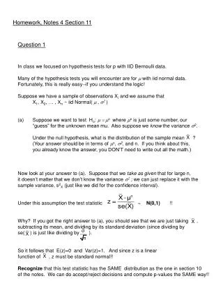
1. Homework, Notes 4 Section 11 Question 1 • In class we focused on hypothesis tests for p with IID Bernoulli data. • Many of the hypothesis tests you will encounter are for mwith iid normal data. • Fortunately, this is really easy--if you understand the logic! • Suppose we have a sample of observations Xi and we assume that • X1, X2, … , Xn ~ iid Normal( m , s2) • Suppose we want to test Ho:m = mo where mo is just some number, our • “guess” for the unknown mean mu. Also suppose we know the variance s2. • Under the null hypothesis, what is the distribution of the sample mean ? • (Your answer should be in terms of mo, s2, and n. If you think about this, • you already know the answer, you DON’T need to write out all the math.) • Now look at your answer to (a). Suppose that we take as given that for large n, • it doesn’t matter that we don’t know the variance s2 ; we can just replace it with the • sample variance, s2X (just like we did for the confidence interval). • Under this assumption the test statistic ~ N(0,1) !! Why? If you got the right answer to (a), you should see that we are just taking , subtracting its mean, and dividing by its standard deviation (since dividing by se( ) is just like dividing by ). So it follows that E(z)=0 and Var(z)=1. And since z is a linear function of , z must be standard normal!! Recognize that this test statistic has the SAME distribution as the one in section 10 of the notes. We can do accept/reject decisions and compute p-values the SAME way!!

2. (b) Let’s look at the Canadian returns data again. • Assuming the returns are iid, write down a 95% confidence interval for m. • (The answer is on slide 49 of your lecture notes, so you don’t have to • do it again if you don’t want to.) • Now test the null hypothesis that m = .01 at the 5% level. • Do you accept or reject? • Using the same data, test the following null hypotheses at the 5% level: • (i) Ho: m= 0 (ii) Ho: m= .018 • For each one, do you accept or reject? • (You can use StatPro to do these tests. Choose Statistical Inference -> • One Sample Analysis… choose “canada” as your variable and check • “hypothesis tests on the mean”. Now pick “two-tailed alternative” and • enter the appropriate claimed value mo for “value under the null”.) Stop and think about this for a minute. A confidence interval and a hypothesis test are two ways of saying what we think about the true value of m. Remember the formula for our 95% CI: Now look at the formula for the test statistic: • We started our hypothesis test by making the “claim” Ho: m = mo . Remember,mo is our “guess” for the value of the unknown quanity, mu. Here’s the punchline: In this problem we can tell immediately whether Ho will be rejected, just by looking at the confidence interval. HOW?

3. Question 2 In the last homework assignment, we constructed a confidence interval for the mean of the Australian returns from our countries data set. As we’ve discussed in class, this confidence interval assumes that the data are iid. We might also be interested in asking whether the data are normally distributed. (a) Construct a time series plot and a historgram of the Australian returns data. Based on this visual evidence, do you think the iid normal model is appropriate? • (b) In StatPro, select Statistical Inference -> Runs Test for Randomness. • StatPro calls it a test for "randomness", what the heck does that mean? • The null hypothesis being tested by the runs test is that the data are iid draws • from some distribution. • Now in StatPro, select Tests for Normality -> Lilliefors Test Here the null • hypothesis is that we are drawing from some normal distribution. This test • assumes the data is iid. • Using StatPro, obtain the p-values associated with each of these tests. • For each null hypothesis, do you reject at the 5% level? • Are the results consistent with your “eyeball” assessment from part (a)? • Give a brief answer, but be specific about what the tests are telling you. (c) Using StatPro, construct the 95% confidence interval for the mean of the Australian returns. Also construct the 95% plug-in predictive interval. What do the outcomes of the tests in part (b) tell us about our confidence interval and our predictive interval? In particular, if you had rejected either or both of the null hypotheses in part (b), would it affect how you interpret the confidence interval? How about the predictive interval?

4. Question 3 In last week’s homework we used a confidence interval to assess the difference between two means. This time let’s use a hypothesis test. Open up the housing data in Excel and click on Sheet 1. This is a sample of homes sold in a given suburban area in a particular year. We are interested in evaluating the following statement: “The mean price of brick houses is the same as the mean price of non-brick houses.” (a) Let mbr = the expected price of a brick house mnon = the expected price of a non-brick house In terms of the two m’s, what is Ho (the null hypothesis we are testing)? (b) In StatPro, select Statistical Inference -> Two Sample Analysis… Choose “Stacked”, select “brick” as your code variable and “price” as your measurement variable. Now click on “Hypothesis test on the difference…”. Leave “two-tailed alternative” selected (this basically means we don’t care whether brick houses or more or less expensive, just whether or not the price is different on average) and use your answer to part (a) to fill in “value under the null”. When StatPro asks where you want the results, choose “to the right of the data”. The p-value in row 18 of your worksheet will then be the p-value for the test of the null hypothesis Ho from part (a). Do you reject the null at the 5% level? About how strong is the evidence? (Like the confidence intervals we looked at in the last problem last week, there are two ways to do the calculation, both of which are described in the book. Both of them give you the same answer.) (c) Now suppose instead of doing a hypothesis test we had made a 95% confidence interval for mbr – mnon (like we did for the beer data last week). Explain how we could have gotten the same reject/fail to reject answer as in (b) by looking at the 95% CI (look back at question #1). (d) The entries in rows 21-22 are from a test of the null hypothesis that the variances of prices are equal for brick houses vs. non-brick houses. Do you reject this null hypothesis at the 5% level?