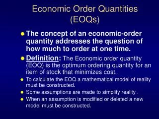
Lecture 23 Order Quantities

1. Lecture 23Order Quantities Books Introduction to Materials Management, Sixth Edition, J. R. Tony Arnold, P.E., CFPIM, CIRM, Fleming College, Emeritus, Stephen N. Chapman, Ph.D., CFPIM, North Carolina State University, Lloyd M. Clive, P.E., CFPIM, Fleming College Operations Management for Competitive Advantage, 11th Edition, by Chase, Jacobs, and Aquilano, 2005, N.Y.: McGraw-Hill/Irwin. Operations Management, 11/E, Jay Heizer, Texas Lutheran University, Barry Render, Graduate School of Business, Rollins College, Prentice Hall

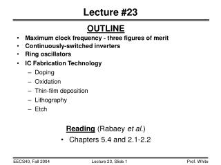
2. Objectives • Objectives of inventory management • Lot size decision • Inventory models • EOQ • Robust model • Reorder point • Production order quantity model • Quantity discount model

3. Objectives of Inventory Management Determine: • How much should be ordered at one time? • When should an order be placed?

4. Lot-Size Decision Rules Lot-for-lot. Order exactly what is needed. Fixed-order quantity. Arbitrary Order “n” periods supply. Satisfy demand for a given period of demand.

5. Inventory Models for Independent Demand Need to determine when and how much to order • Basic economic order quantity • Production order quantity • Quantity discount model

6. Basic EOQ Model Important assumptions Demand is known, constant, and independent Lead time is known and constant Receipt of inventory is instantaneous and complete Quantity discounts are not possible Only variable costs are setup and holding Stockouts can be completely avoided

7. Inventory Usage Over Time Average inventory on hand Q 2 Usage rate Inventory level Minimum inventory 0 Time Order quantity = Q (maximum inventory level)

8. Minimizing Costs Curve for total cost of holding and setup Minimum total cost Holding cost curve Annual cost Setup (or order) cost curve Order quantity Optimal order quantity (Q*) Objective is to minimize total costs

9. The EOQ Model D Q Annual setup cost = S Annual demand Number of units in each order Setup or order cost per order = = (S) D Q Q = Number of pieces per order Q* = Optimal number of pieces per order (EOQ) D = Annual demand in units for the inventory item S = Setup or ordering cost for each order H = Holding or carrying cost per unit per year Annual setup cost = (Number of orders placed per year) x (Setup or order cost per order)

10. The EOQ Model D Q Annual setup cost = S Annual holding cost = H Order quantity 2 = (Holding cost per unit per year) = (H) Q 2 Q 2 Q = Number of pieces per order Q* = Optimal number of pieces per order (EOQ) D = Annual demand in units for the inventory item S = Setup or ordering cost for each order H = Holding or carrying cost per unit per year Annual holding cost = (Average inventory level) x (Holding cost per unit per year)

11. The EOQ Model D Q Annual setup cost = S Annual holding cost = H Q 2 D Q S = H 2DS = Q2H Q2 = 2DS/H Q* = 2DS/H Q 2 Q = Number of pieces per order Q* = Optimal number of pieces per order (EOQ) D = Annual demand in units for the inventory item S = Setup or ordering cost for each order H = Holding or carrying cost per unit per year Optimal order quantity is found when annual setup cost equals annual holding cost Solving for Q*

12. An EOQ Example 2DS H Q* = 2(1,000)(10) 0.50 Q* = = 40,000 = 200 units Determine optimal number of needles to order D = 1,000 units S = $10 per order H = $.50 per unit per year

13. An EOQ Example Expected number of orders Demand Order quantity D Q* = N = = 1,000 200 N = = 5 orders per year Determine optimal number of needles to order D = 1,000 units Q* = 200 units S = $10 per order H = $.50 per unit per year

14. An EOQ Example Number of working days per year N Expected time between orders = T = 250 5 T = = 50 days between orders Determine optimal number of needles to order D = 1,000 units Q* = 200 units S = $10 per order N = 5 orders per year H = $.50 per unit per year

15. An EOQ Example Q 2 D Q 200 2 TC = S + H 1,000 200 TC = ($10) + ($.50) Determine optimal number of needles to order D = 1,000 units Q* = 200 units S = $10 per order N = 5 orders per year H = $.50 per unit per year T = 50 days Total annual cost = Setup cost + Holding cost TC = (5)($10) + (100)($.50) = $50 + $50 = $100

16. Robust Model • The EOQ model is robust • It works even if all parameters and assumptions are not met • The total cost curve is relatively flat in the area of the EOQ

17. An EOQ Example 1,500 units Q 2 D Q 200 2 TC = S + H 1,500 200 TC = ($10) + ($.50) = $75 + $50 = $125 Management underestimated demand by 50% D = 1,000 units Q* = 200 units S = $10 per order N = 5 orders per year H = $.50 per unit per year T = 50 days Total annual cost increases by only 25%

18. An EOQ Example 1,500 units 244.9 2 TC = ($10) + ($.50) Q 2 D Q TC = S + H 1,500 244.9 Actual EOQ for new demand is 244.9 units D = 1,000 units Q* = 244.9 units S = $10 per order N = 5 orders per year H = $.50 per unit per year T = 50 days Only 2% less than the total cost of $125 when the order quantity was 200 TC = $61.24 + $61.24 = $122.48

19. Reorder Points Lead time for a new order in days ROP = Demand per day D Number of working days in a year d = • EOQ answers the “how much” question • The reorder point (ROP) tells when to order = d x L

20. Reorder Point Curve Q* Slope = units/day = d Inventory level (units) ROP (units) Time (days) Lead time = L

21. Reorder Point Example D Number of working days in a year d = Demand = 8,000 iPods per year 250 working day year Lead time for orders is 3 working days = 8,000/250 = 32 units ROP = d x L = 32 units per day x 3 days = 96 units

22. Production Order Quantity Model • Used when inventory builds up over a period of time after an order is placed • Used when units are produced and sold simultaneously

23. Production Order Quantity Model Part of inventory cycle during which production (and usage) is taking place Demand part of cycle with no production Inventory level Maximum inventory t Time

24. Production Order Quantity Model = (Average inventory level) x Annual inventory holding cost Annual inventory level Holding cost per unit per year = (Maximum inventory level)/2 Maximum inventory level Total produced during the production run Total used during the production run = – = pt – dt Q = Number of pieces per order p = Daily production rate H = Holding cost per unit per year d = Daily demand/usage rate t = Length of the production run in days

25. Production Order Quantity Model = – = pt – dt = p – d = Q 1 – Maximum inventory level Maximum inventory level Total produced during the production run Total used during the production run Q p Q p d p d p Maximum inventory level 2 Q 2 Holding cost = (H) = 1 – H Q = Number of pieces per order p = Daily production rate H = Holding cost per unit per year d = Daily demand/usage rate t = Length of the production run in days However, Q = total produced = pt ; thus t = Q/p

26. Production Order Quantity Model Setup cost = (D/Q)S Holding cost = HQ[1 - (d/p)] 1 2 1 2 (D/Q)S = HQ[1 - (d/p)] Q2 = 2DS H[1 - (d/p)] 2DS H[1 - (d/p)] Q* = p Q = Number of pieces per order p = Daily production rate H = Holding cost per unit per year d = Daily demand/usage rate D = Annual demand

27. Production Order Quantity Example 2(1,000)(10) 0.50[1 - (4/8)] Q* = = 80,000 = 282.8 or 283 hubcaps 2DS H[1 - (d/p)] Q* = D = 1,000 units p = 8 units per day S = $10 d = 4 units per day H = $0.50 per unit per year

28. Production Order Quantity Model 1,000 250 D Number of days the plant is in operation d = 4 = = 2DS Q* = annual demand rate annual production rate H 1 – Note: When annual data are used the equation becomes

29. EPQ Problem: HP Ltd. Produces premium plant food in 50# bags. Demand is 100,000 lbs/week. They operate 50 wks/year; HP produces 250,000 lbs/week. Setup cost is $200 and the annual holding cost rate is $.55/bag. Calculate the EPQ. Determine the maximum inventory level. Calculate the total cost of using the EPQ policy.

30. EPQ Problem Solution

31. Quantity Discount Models Q 2 TC = S + H + PD D Q • Reduced prices are often available when larger quantities are purchased • Trade-off is between reduced product cost and increased holding cost Total cost = Setup cost + Holding cost + Product cost

32. Quantity Discount Models A typical quantity discount schedule

33. Quantity Discount Models Steps in analyzing a quantity discount For each discount, calculate Q* If Q* for a discount doesn’t qualify, choose the smallest possible order size to get the discount Compute the total cost for each Q* or adjusted value from Step 2 Select the Q* that gives the lowest total cost

34. Quantity Discount Models Total cost curve for discount 2 Total cost curve for discount 1 Total cost $ Total cost curve for discount 3 b a Q* for discount 2 is below the allowable range at point a and must be adjusted upward to 1,000 units at point b 1st price break 2nd price break 0 1,000 2,000 Order quantity

35. Quantity Discount Example 2(5,000)(49) (.2)(5.00) 2(5,000)(49) (.2)(4.80) 2(5,000)(49) (.2)(4.75) Q1* = = 700 cars/order Q2* = = 714 cars/order Q3* = = 718 cars/order 2DS IP Q* = Calculate Q* for every discount

36. Quantity Discount Example 2(5,000)(49) (.2)(5.00) 2(5,000)(49) (.2)(4.80) 2(5,000)(49) (.2)(4.75) Q1* = = 700 cars/order Q2* = = 714 cars/order Q3* = = 718 cars/order 2DS IP Q* = 1,000 — adjusted 2,000 — adjusted Calculate Q* for every discount

37. Quantity Discount Example Choose the price and quantity that gives the lowest total cost Buy 1,000 units at $4.80 per unit

38. Quantity Discount Example: Collin’s Sport store is considering going to a different hat supplier. The present supplier charges $10/hat and requires minimum quantities of 490 hats. The annual demand is 12,000 hats, the ordering cost is $20, and the inventory carrying cost is 20% of the hat cost, a new supplier is offering hats at $9 in lots of 4000. Who should he buy from? • EOQ at lowest price $9. Is it feasible? • Since the EOQ of 516 is not feasible, calculate the total cost (C) for each price to make the decision • 4000 hats at $9 each saves $19,320 annually. Space?

39. End of Lecture 23