Download
1 / 22
220 likes | 357 Vues
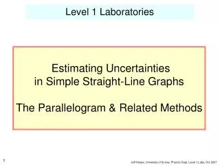
This document outlines the Parallelogram Method for estimating uncertainties in the gradient and intercept of linear graphs. It details the procedure to draw extreme lines, derive the best-fit line, and calculate error margins based on the area under a normal distribution curve. The guide provides illustrations and example calculations to aid understanding, emphasizing the relevance of proper data representation and error analysis in experimental physics.

E N D
Level 1 Laboratories Estimating Uncertainties in Simple Straight-Line Graphs The Parallelogram & Related Methods 1 Jeff Hosea, University of Surrey, Physics Dept, Level 1 Labs, Oct 2007
20 15 10 5 0 0 5 10 15 Example of Parallelogram Method to obtain errors in gradient & intercept (dimensionless) y x (dimensionless) Figure 1 : Give the graph a title to which you can refer ! & Add a descriptive caption. Blah, blah …… 2 Jeff Hosea : University of Surrey, Physics Dept, Level 1 Labs, Oct 2007
gradient m [ e.g. here m= 0.59 ] intercept c [ e.g. here c= 6.5 ] Example of Parallelogram Method to obtain errors in gradient & intercept 20 Estimate ”best fit” line 15 y (dimensionless) 10 5 0 0 5 10 15 x (dimensionless) 3 Jeff Hosea : University of Surrey, Physics Dept, Level 1 Labs, Oct 2007
2 68.3% of area under Normal curve Example of Parallelogram Method to obtain errors in gradient & intercept 20 Draw 2 lines parallel to best line so as to enclose roughly 2/3 of data points 15 y (dimensionless) 10 5 0 0 5 10 15 x (dimensionless) Why 2/3? - It’s because we assume the data obey a Normal Distribution in which there is a 68.3% ( 66.7% = 2/3) confidence that the “true” value lies within of the measured value 4 Jeff Hosea : University of Surrey, Physics Dept, Level 1 Labs, Oct 2007
Min gradient mL Max intercept CH Min intercept CL Max gradient mH Example of Parallelogram Method to obtain errors in gradient & intercept 20 Draw “extreme lines” between opposite corners of parallelogram 15 10 5 0 0 5 10 15 x (dimensionless) 5 Jeff Hosea : University of Surrey, Physics Dept, Level 1 Labs, Oct 2007
Min gradient mL Final Results including errors Min intercept CL Max intercept CH Max gradient mH Example of Parallelogram Method to obtain errors in gradient & intercept 20 Draw “extreme lines” between opposite corners of parallelogram 15 10 5 0 0 5 10 15 x (dimensionless) 6 Jeff Hosea : University of Surrey, Physics Dept, Level 1 Labs, Oct 2007
Example of Parallelogram Method to obtain errors in gradient & intercept 20 Add expt. “error bars” 15 y (dimensionless) 10 5 0 0 5 10 15 x (dimensionless) NB : these error bars are estimated from the scatter in the data. Here, they play no part in getting the errors in the gradient and intercept. 7 Jeff Hosea : University of Surrey, Physics Dept, Level 1 Labs, Oct 2007
20 15 y (dimensionless) 10 5 0 0 5 10 15 x (dimensionless) Recommended final appearance of graph for Diary or Reports, if using Parallelogram Method Figure 1 : Descriptive caption. Blah, blah …… 8 Jeff Hosea : University of Surrey, Physics Dept, Level 1 Labs, Oct 2007
Plot the experimental points (x, ydata) y x What if the scatter is so small that it is difficult to draw the max. and min. lines by eye? Method 2 :Modified Parallelogram Method 9
Draw the best fit line and determine equation • yfit = m1x + c1 y x What if the scatter is so small that it is difficult to draw the max. and min. lines by eye? Method 2 :Modified Parallelogram Method • Plot the experimental points (x, ydata) 10
y • The small difference • (ydata – yfit ) will be dominated by the random scatter x What if the scatter is so small that it is difficult to draw the max. and min. lines by eye? Method 2 :Modified Parallelogram Method • Plot the experimental points (x, ydata) • Draw the best fit line and determine equation • yfit = m1x + c1 0 11
y x • Replot (ydata – yfit ) on an expanded scale. 0 (ydata – yfit) x What if the scatter is so small that it is difficult to draw the max. and min. lines by eye? Method 2 :Modified Parallelogram Method • Plot the experimental points (x, ydata) • Draw the best fit line and determine equation • yfit = m1x + c1 • The small difference • (ydata – yfit ) will be dominated by the random scatter 0 12
y x • Fit the best line • (ydata – yfit ) = m2x + c2 What if the scatter is so small that it is difficult to draw the max. and min. lines by eye? Method 2 :Modified Parallelogram Method • Plot the experimental points (x, ydata) • Draw the best fit line and determine equation • yfit = m1x + c1 • The small difference • (ydata – yfit ) will be dominated by the random scatter 0 • Replot (ydata – yfit ) on an expanded scale. 0 (ydata – yfit) 13 x
y x • Form the parallelogram enclosing 2/3 of points What if the scatter is so small that it is difficult to draw the max. and min. lines by eye? Method 2 :Modified Parallelogram Method • Plot the experimental points (x, ydata) • Draw the best fit line and determine equation • yfit = m1x + c1 • The small difference • (ydata – yfit ) will be dominated by the random scatter 0 • Replot (ydata – yfit ) on an expanded scale. • Fit the best line • (ydata – yfit ) = m2x + c2 0 (ydata – yfit) 14 x
y x • Use the extreme lines to find the max and min values of m2and c2 What if the scatter is so small that it is difficult to draw the max. and min. lines by eye? Method 2 :Modified Parallelogram Method • Plot the experimental points (x, ydata) • Draw the best fit line and determine equation • yfit = m1x + c1 • The small difference • (ydata – yfit ) will be dominated by the random scatter 0 • Replot (ydata – yfit ) on an expanded scale. • Fit the best line • (ydata – yfit ) = m2x + c2 0 (ydata – yfit) • Form the parallelogram enclosing 2/3 of points 15 x
Final Results including errors y x What if the scatter is so small that it is difficult to draw the max. and min. lines by eye? Method 2 :Modified Parallelogram Method • Plot the experimental points (x, ydata) • Draw the best fit line and determine equation • yfit = m1x + c1 • The small difference • (ydata – yfit ) will be dominated by the random scatter 0 • Replot (ydata – yfit ) on an expanded scale. • Fit the best line • (ydata – yfit ) = m2x + c2 0 (ydata – yfit) • Form the parallelogram enclosing 2/3 of points • Use the extreme lines to find the max and min values of m2and c2 16 x
y 0 x There is another method commonly used when the scatter is small Method 3 :Using Predetermined Error Bars (e.g. by multiple measurements at a single value of x) 17 Jeff Hosea : University of Surrey, Physics Dept, Level 1 Labs, Oct 2007
Add predetermined error bars to the plotted points y x There is another method commonly used when the scatter is small Method 3 :Using Predetermined Error Bars (e.g. by multiple measurements at a single value of x) 0 18 Jeff Hosea : University of Surrey, Physics Dept, Level 1 Labs, Oct 2007
Draw best line through points • (if predetermined error is consistent with the scatter in the points, the line should go through ~2/3 of error bars & miss remaining ~1/3 ) y x There is another method commonly used when the scatter is small Method 3 :Using Predetermined Error Bars (e.g. by multiple measurements at a single value of x) • Add predetermined error bars to the plotted points 0 19 Jeff Hosea : University of Surrey, Physics Dept, Level 1 Labs, Oct 2007
y • Put in extreme lines so as to still pass through ~2/3 of error bars x There is another method commonly used when the scatter is small Method 3 :Using Predetermined Error Bars (e.g. by multiple measurements at a single value of x) • Add predetermined error bars to the plotted points • Draw best line through points • (if predetermined error is consistent with the scatter in the points, the line should go through ~2/3 of error bars & miss remaining ~1/3 ) 0 20 Jeff Hosea : University of Surrey, Physics Dept, Level 1 Labs, Oct 2007
Final Results including errors y 0 x There is another method commonly used when the scatter is small Method 3 :Using Predetermined Error Bars (e.g. by multiple measurements at a single value of x) • Add predetermined error bars to the plotted points • Draw best line through points • (if predetermined error is consistent with the scatter in the points, the line should go through ~2/3 of error bars & miss remaining ~1/3 ) • Put in extreme lines so as to still pass through ~2/3 of error bars 21 Jeff Hosea : University of Surrey, Physics Dept, Level 1 Labs, Oct 2007
Caution with Method 3 y 0 x • If the “scatter” in plotted data looks different to the size of error bars (much smaller or larger), something has gone wrong! • Example shows all y-axis error bars of same length. This might not be true in any given case, so do not assume this unless you have confirmed it! • Example also shows no error bars on the horizontal x-axis : there might be errors in this direction too! 22 Jeff Hosea : University of Surrey, Physics Dept, Level 1 Labs, Oct 2007