Download
1 / 38
380 likes | 408 Vues
Use machine learning to compute abstraction conditions from traces to create abstractions by generalizing simulation data.

E N D
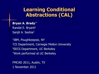
Learning Conditional Abstractions (CAL) Bryan A. Brady1* Randal E. Bryant2 SanjitA. Seshia3 1IBM, Poughkeepsie, NY 2CS Department, Carnegie Mellon University 3EECS Department, UC Berkeley *Work performed at UC Berkeley FMCAD 2011, Austin, TX 1 November 2011
Learning Conditional Abstractions Learning Conditional Abstractions (CAL): Use machine learning from traces to compute abstraction conditions. Philosophy: Create abstractions by generalizing simulation data.
Abstraction Levels in FV • Term-level verifiers • SMT-based verifiers (e.g., UCLID) • Able to scale to much more complex systems • How to decide what to abstract? Term Level ??? Designs are typically at this level Bit Vector Level Bit Blast • Most tools operate at this level • Model checkers • Equivalence checkers • Capacity limited by • State bits • Details of bit-manipulations Bit Level
Motivating Example • Equivalence/Refinement Checking = fB fA • Difficult to reason about some operators • Multiply, Divide • Modulo, Power Design B Design A • Term-level abstraction • Replace bit-vector operators with uninterpreted functions • Represent data with arbitrary encoding x1 x2 xn f(...) * / % ^
Term-Level Abstraction Fully uninterpreted Example Precise, word-level instr := JMP 1234 out1 out2 1 0 out1:= 1234 UF ALU out2:= 0 16 = Need to partially abstract 16 16 16 20 4 JMP instr 19 15 0 instr
Term-Level Abstraction Fully uninterpreted Precise, word-level Partially-interpreted out out out 1 1 0 0 UF ALU 16 16 UF = = 16 16 16 16 16 20 4 4 JMP JMP instr 19 15 0 19 15 0 instr instr
Term-Level Abstraction • Manual Abstraction • Requires intimate knowledge of design • Multiple models of same design • Spurious counter-examples Perform Abstraction RTL Verification Model • Automatic Abstraction • How to choose the right level of abstraction • Some blocks require conditional abstraction • Often requires many iterations of abstraction refinement
Outline • Motivation • Related work • Background • The CAL Approach • Illustrative Example • Results • Conclusion
Outline • Motivation • Related work • Background • ATLAS • Conditional Abstraction • The CAL Approach • Illustrative Example • Results • Conclusion
Background: The ATLAS Approach • Hybrid approach • Phase 1: Identify abstraction candidates with random simulation • Phase 2: Use dataflow analysis to compute conditions under which it is precise to abstract • Phase 3: Generate abstracted model Compute Abstraction Conditions Identify Abstraction Candidates Generate Abstracted Model
Identify Abstraction Candidates • Find isomorphic sub-circuits (fblocks) • Modules, functions = fA fB Design B Design A Replace each fblock with a random function, over the inputs of the fblock a a a RFa RFa a a a b RFb b b b b RFb b c RFc RFc c c c c c • Verify via simulation: • Check original property for N different random functions x1 x2 xn
Identify Abstraction Candidates Do not abstract fblocks that fail in some fraction of simulations = fA fB Intuition: fblocks that can not be abstracted will fail when replaced with random functions. Design B Design A a a a a Replace remaining fblocks with partially-abstract functions and compute conditions under which the fblock is modeled precisely b UFb UFb b c c c c Intuition: fblocks can contain a corner case that random simulation didn’t explore x1 x2 xn
Modeling with Uninterpreted Functions interpretation condition g = fA fB c 1 0 Design B Design A UF b a a a a UFb b UFb b c c c c x1 x2 xn y1 y2 yn
Interpretation Conditions Problem: Compute interpretation condition c(x)such that∀x.f1⇔f2 D1,D2 : word-level designs T1,T2 : term-level models x : input signals c : interpretation condition = = f1 f2 Trivial case, model precisely: c = true Ideal case, fully abstract: c = false T2 D2 D1 T1 Realistic case, we need to solve: ∃c ≠ true s.t. ∀x.f1⇔f2 This problem is NP-hard, so we use heuristics to compute c x c
Outline • Motivation • Related work • Background • The CAL Approach • Illustrative Example • Results • Conclusion
Related Work Previous work related to Learning and Abstraction • Learning Abstractions for Model Checking • Anubhav Gupta, Ph.D. thesis, CMU, 2006 • Localization abstraction: learn the variables to make visible • Our approach: • Learn when to apply function abstraction
The CAL Approach • CAL = Machine Learning + CEGAR • Identify abstraction candidates with random simulation • Perform unconditional abstraction • If spurious counterexamples arise, use machine learning to refine abstraction by computing abstraction conditions • Repeat Step 3 until Valid or real counterexample
The CAL Approach Random Simulation RTL Modules to Abstract Abstraction Conditions Simulation Traces Generate Term-Level Model Invoke Verifier Valid? Yes Done Learn Abstraction Conditions Counter example Spurious? Generate Similar Traces No Yes No Done
Use of Machine Learning Learning Algorithm Concept (classifier) Examples (positive/negative) In our setting: Learning Algorithm Interpretation condition Simulation traces (correct / failing)
Important Considerations in Learning • How to generate traces for learning? • What are the relevant features? • Random simulations: using random functions in place of UFs • Counterexamples • Inputs to functional block being abstracted • Signals corresponding to “unit of work” being processed
Generating Traces: Witnesses Modified version of random simulation = Replace allmodules that are being abstracted with RF at same time fA fB Design B Design A Verify via simulation for N iterations a a RFa a a a RFa a RFa RFa RFb b RFb b b b b b Log signals for each passing simulation run RFb RFb c RFc c c c c RFc c RFc RFc • Important note: initial state selected randomly or based on a testbench x1 x2 xn
Generating Traces: Similar Counterexamples Replace modules that are being abstracted with RF, one by one = fA fB Verify via simulation for N iterations Design B Design A Log signals for each failing simulation run a RFa RFa a a a a a b RFb RFb b b b b b Repeat this process for each fblock that is being abstracted c c RFc c c c RFc c • Important note: initial state set to be consistent with the original counterexample for each verification run x1 x2 xn
Feature Selection Heuristics • Include inputs to the fblock being abstracted • Advantage: automatic, direct relevance • Disadvantage: might not be enough • Include signals encoding the “unit-of-work” being processed by the design • Example: an instruction, a packet, etc. • Advantage: often times the “unit-of-work” has direct impact on whether or not to abstract • Disadvantage: might require limited human guidance
Outline • Motivation • Related work • Background • The CAL Approach • Illustrative Example • Results • Conclusion
Learning Example Example: Y86 processor design Abstraction: ALU module Unconditional abstraction Counterexample Sample data set bad,7,0,1,0 bad,7,0,1,0 bad,7,0,1,0 bad,7,0,1,0 bad,7,0,1,0 good,11,0,1,-1 good,11,0,1,1 good,6,3,-1,-1 good,6,6,-1,1 good,9,0,1,1 {0,1,...,15} Attribute, instr, aluOp, argA, argB Abstract interpretation: x < 0 -1 x = 0 0 x > 0 1 {Good, Bad} {-1,0,1}
Learning Example Example: Y86 processor design Abstraction: ALU module Unconditional abstraction Counterexample Sample data set bad,7,0,1,0 bad,7,0,1,0 bad,7,0,1,0 bad,7,0,1,0 bad,7,0,1,0 good,11,0,1,-1 good,11,0,1,1 good,6,3,-1,-1 good,6,6,-1,1 good,9,0,1,1 Feature selection based on “unit-of-work” Interpretation condition learned: InstrE = JXX ∧ b = 0 Verification succeeds when above interpretation condition is used!
Learning Example Example: Y86 processor design Abstraction: ALU module Unconditional abstraction Counterexample Sample data set bad,0,1,0 bad,0,1,0 bad,0,1,0 bad,0,1,0 bad,0,1,0 good,0,1,-1 good,0,1,1 good,3,-1,-1 good,6,-1,1 good,0,1,1 If feature selection is based on fblock inputs only... Interpretation condition learned: true Recall that this means we always interpret! Poor decision tree results from reasonable design decision. More information needed.
Outline • Motivation • Related work • Background • The CAL Approach • Illustrative Example • Results • Conclusion
Experiments/Benchmarks • Pipeline fragment: • Abstract ALU • JUMP must be modeled precisely. • ATLAS: Automatic Term-Level Abstraction of RTL Designs. B. A. Brady, R. E. Bryant, S. A. Seshia, J. W. O’Leary. MEMOCODE 2010 • Low-power Multiplier: • Performs equivalence checking between two versions of a multiplier • One is a typical multiplier • The “low-power” version shuts down the multiplier and uses a shifter when one of the operands is a power of 2 • Low-Power Verification with Term-Level Abstraction. B. A. Brady. TECHCON ‘10 • Y86: • Correspondence checking of 5-stage microprocessor • Multiple design variations • Computer Systems: A Programmer’s Perspective. Prentice-Hall, 2002. R. E. Bryant and D. R. O’Hallaron.
Experiments/Benchmarks Pipeline fragment Low-Power Multiplier
Experiments/Benchmarks Y86: BTFNT Y86: NT
Outline • Motivation • Related work • Background • The CAL Approach • Illustrative Example • Results • Conclusion
Summary / Future Work Summary • Use machine learning + CEGAR to compute conditional function abstractions • Outperforms purely bit-level techniques Future Work • Better feature selection: picking “unit-of-work” signals • Investigate using different abstraction conditions for different instantiations of the same fblock. • Apply to software • Investigate interactions between abstractions
NP-Hard 0 1 0 1 Need to interpret MULT when f(x1,x2,...,xn) = true Checking satisfiability off(x1,x2,...,xn) is NP-Hard = MULT MULT +2 +5 +1 +10 f ... x1 x2 xn x 0
Term-Level Abstraction Function Abstraction: Represent functional units with uninterpreted functions f ALU ALU • Data Abstraction: • Represent data with arbitrary integer values • No specific encoding x0 x1 x xn-1


![Computer Assisted Learning [CAL]](https://cdn2.slideserve.com/3962806/slide1-dt.jpg)