Microsoft Excel 2010
Microsoft Excel 2010. Presented by Connie Lanier University of New Orleans TRAC. Filtering Data. Select the Filter button in the Editing group of the Data tab or Select the Filter button in the Editing group of the Home tab, Select the Sort & Filter button


Microsoft Excel 2010
E N D
Presentation Transcript
Microsoft Excel 2010 Presented by Connie Lanier University of New Orleans TRAC
Filtering Data • Select the Filter button in the Editing group of the Data tab • or • Select the Filter button in the Editing group of the Hometab, • Select the Sort & Filterbutton • Select the Filter option from the pull down menu
Filtering Facts • Narrows down data • Data is not changed • Hides rows that do not met the criteria • Apply multiple criteria • Filter text, numbers, and dates • Filter by cell color or font color
Subtotal Function • Very useful when working with Filtered Data • Ignores hidden rows that result from the Filter • Calculations are only applied to visible data • AutoSum button uses the Subtotal function when data is filtered • Math and Trig Function
Subtotal Wizard • Efficient way to summarize data • Adds subtotal rows by each group as well as a grand total • Summarize data must be sorted by the category group • Creates three outlined levels
Subtotal Wizard • Select a cell in the Category column. • Select the Sort A to Z button located on the Data tab. • Next, select the Subtotal button located in the Data tab in the Outline group. The Subtotal dialog box will appear. • Fill in the Subtotal dialog box. Make sure that the Replace Current Subtotals and Summary Below Data options are checked. • Single-click on the OK button.
Subtotal Dialog Box • Note that the data list should be sorted by the Customer column before selecting the Subtotal button. • This column is also referred to as the category column. • In this example, grouped by Customer and summed by Amount Due column.
Pivot Tables • Special type of summary table • Great for summarizing data • Summary can easily be changed on the fly • Exclusive to Microsoft Excel
Preparing the Data • Make sure the list is well organized. • Make sure the first row of the list contains column headings. The column headings will be used as field names in the report. • Make sure each column of data contains similar items. For example, put text in one column and numeric values in another column. • Delete all subtotals and grand totals from the worksheet.
Creating a Pivot Table • Single-click on any cell in the list or database. • Select Pivot Table button in the Insert tab. The Create Pivot Table dialog box appears. • Double check table range. • Select New Worksheet option. • Single-click on the Ok button. The PivotTable Field List opens up and the PivotTable tools tabs become available. • From the Pivot table field list, check fields to appear in the Pivot table report.
Pivot Table Example • In the following example, the Pivot Table will summarize the sales data of each sales person in a company. • Each sales person reports the number of cases of Doodads, Gizmos, Gadgets and Trinkets they sell each quarter. • A report is needed that you can easily display how many cases of each where sold.
Customizing a Pivot Table • Minor Cosmetic Changes—Changing blanks to zeros, adjusting the number format, renaming a field. Although these changes are minor, they are common and affect almost every pivot table that you create. • Layout Changes—Comparing three possible layouts, showing/hiding subtotals and totals. • Major Cosmetic Changes—Using table styles to quickly format the table. • Summary Calculation—Changing from Sum to Count, Min, Max, and more. If you have a table that defaults to Count of Revenue instead of Sum of Revenue, you need to visit this section. • Advanced Calculation—Using settings to show data as a running total, % of total, and more.
Design Tab - Layout Changes • Subtotals—Moves subtotals to the top or bottom of each group, or turns them off. • Grand Totals—Turns the grand totals on or off for rows and columns. • Report Layout—Uses the Compact, Outline, or Tabular forms. • Blank Rows—Inserts or removes blank lines after each group.
Pivot Tables and Slicers • A new feature called Slicer is an easy way to filter the data in Pivot Tables. • When a slicer is inserted, buttons are used to filter the data and display what is needed. • Slicers make it easy to see which filters are applied. • Slicers are graphical objects that can be moved, sized and deleted as needed.
Using Slicers • Select a cell in the Pivot Table. • Select Insert tab. • Single-click on the Slicer button in the Filter group. • Select the field from the Insert Slicers dialog box. • Then single-click on the OK button.
Text Functions • Left Function • LEFT returns the first character or characters in a text string, based on the number of characters you specify. • Right Function • RIGHT returns the last character or characters in a text string, based on the number of characters you specify. • Mid Function • MID returns a specific number of characters from a text string, starting at the position you specify, based on the number of characters you specify. Just like the LEFT function it starts counting from the first character.
Text Functions • Upper Function • UPPER function converts the text to all uppercase letters. • Lower Function • LOWER function converts the text to all lowercase letters. • Proper Function • Properfunction capitalizes the first letter in each word.
An Example • Cell B6 =UPPER(A6) • Cell C6 =LOWER(A6) • Cell D6 =PROPER(A6)
Lookup & Reference Functions • Extracts data from a list of values • Referred to as a Lookup Table • VLOOKUP • Vertical Table • Table is arranged by Columns • HLOOKUP • Horizontal Table • Table is arranged by Rows • LOOKUP • Similar to VLOOKUP
VLOOKUP FUNCTION Example of a Lookup Table • 1st column must be a unique identifier • Numeric data should be sorted in Ascending order • Can contain in number of columns • May be any type of data
VLOOKUP Dialog Box • Lookup_value – Location of Unique Identifier • Table_arrary – Location of the database or list • Col_index_num – Specifies which piece of information to extract from the Lookup table • Range_lookup – Optional – Specifies whether looking for an exact match or range of values
LOOKUP Function • Two Forms • Vector • Used with a large list of values to look up • Used if values may change over time • Array • Used with a small list of values • Used if values remain constant over time • Alternative to the IF function
LOOKUP Dialog Box • Lookup_value • A value that LOOKUP searches for in the first vector. It can be a number, text, a logical value, or a name or reference that refers to a value. • Lookup_vector • A range that contains only one row or one column. The values in lookup_vector can be text, numbers, or logical values. This must be ascending order. • Result_vector • A range that contains only one row or column. The result_vector argument must be the same size as lookup_vector.
Freeze Panes • Used to keep rows and/or columns visible while scrolling through the Worksheet • Especially useful with large worksheets • Located in the View tab – Window group
Freeze Panes Options • Freeze Top Row • Freezes the 1st visible row • Freeze First Column • Freezes the 1st visible column • Freeze Panes • Freeze both rows and columns
View Side by Side • A side-by-side comparison of two files • Located in View tab – Window group • If more than two files are open, Excel opens the Compare Side by Side dialog box with a list of the other open files • Synchronous Scrolling is on by default
Conditional Formatting • Apply formatting to one or more cells based on the value of the cell • Highlight interesting or unusual cell values, and visualize the data using formatting like font and cell colors • Located in the Home tab – Styles group
Conditional Formatting ExampleEmployees with 30or more years of service shaded in red
IF Function • Formulas tab – Function Library group • Logical library button • Decision Making type function • Nest up to 64 IF functions
Date & Time Data • Date and Time data have value • Easily perform mathematical calculations • Excel’s date and time systems are based upon a serial number
Date & Time Shortcut Keys • CTRL + ; • Inserts the current computer date • Not updateable • CTRL + SHIFT + : • Inserts the current computer time • Not updateable
Date & Time Functions Formulas tab – Function Library group Date & Time library button • TODAY • Inserts the current computer date • Updateable • NOW • Inserts the current computer date and time • Updateable
Date Functions • YEAR • Extracts the Year portion of a date • MONTH • Extracts the Month portion of a date • DAY • Extracts the Day portion of a date
UNO – TRACContact Information • Phone Number: (504) 280-5701 • TRAC Web Site: http://trac.uno.edu/ • Facebook: https://www.facebook.com/trac.uno.edu • Personal Computer Training contact: • Connie Lanier at clanier@uno.edu or 504 280-5701 • Residential Lodging and Meeting Rooms Contact: • Naomi Moore at nmmoore@uno.edu or 504-280-5701
Background Info The University of New Orleans Training, Resource and Assistive-technology Center (TRAC) provides quality services to persons with disabilities, rehabilitation professionals, educators and employers. Established in 1986, by Oliver St. Pé this program has grown and responded to the changing needs of the community. UNO TRAC has built a solid reputation for its innovative training programs and community outreach efforts. The Center is recognized as a valuable resource statewide, nationally and internationally on disability issues. In 1996, the Center opened the doors of its new facility on the Lakefront Campus. UNO TRAC Center is a training, evaluation, conference, administrative and short-term residential facility.
Personal Computer Training • For over 20 years, the University of New Orleans has provided quality training to public sector employees throughout Louisiana. • We can bring the classroom to you. Our experienced instructors can bring computers on site to provide convenient, effective training. • TRAC staff conducts training in the latest software like Microsoft Office. • Staff also can design customized computer training courses to meet the needs of your agency.
Conference & Meeting Rooms • Affordable, academic setting for a conference or meeting, UNO TRAC can meet your needs • TRAC is an accessible facility with features accommodating people with disabilities. • Free parking is available for conference participants and guests. • Catering is available through ARAMARK, located on the campus.