Segmentation
Segmentation. CIS 465 – Topics in Computer Vision Dr. Ramprasad Bala UMass Dartmouth. Assignment 2. Isolate the objects in the image by thresholding Simple enough?. Thresholding Detection Methods.

Segmentation
E N D
Presentation Transcript
Segmentation CIS 465 – Topics in Computer Vision Dr. Ramprasad Bala UMass Dartmouth
Assignment 2 • Isolate the objects in the image by thresholding • Simple enough?
Thresholding Detection Methods • If some property of an image after segmentation is known a priori, the task of threshold selection is simplified, since the threshold is chosen to ensure this property is satisfied. • A printed text sheet may be an example if we know that characters of the text cover 1/p of the sheet area.
Thresholding detection methods • P-tile-thresholding • choose a threshold T (based on the image histogram) such that 1/p of the image area has gray values less than T and the rest has gray values larger than T • in text segmentation, prior information about the ratio between the sheet area and character area can be used • if such a priori information is not available - another property, for example the average width of lines in drawings, etc. can be used - the threshold can be determined to provide the required line width in the segmented image
More complex methods of threshold detection • based on histogram shape analysis • bimodal histogram - if objects have approximately the same gray level that differs from the gray level of the background
Auto-thresholding • Threshold-based segmentation ... minimum segmentation error requirements • it makes intuitive sense to determine the threshold as the gray level that has a minimum histogram value between the two mentioned maxima • multimodal histogram - more thresholds may be determined at minima between any two maxima.
Bimodality of histograms • to decide if a histogram is bimodal or multimodal may not be so simple in reality • it is often impossible to interpret the significance of local histogram maxima
Bimodal histogram threshold detection algorithms • Mode method - find the highest local maxima first and detect the threshold as a minimum between them • to avoid detection of two local maxima belonging to the same global maximum, a minimum distance in gray levels between these maxima is usually required • or techniques to smooth histograms are applied • Histogram bimodality itself does not guarantee correct threshold segmentation
Optimal thresholding • Based on approximation of the histogram of an image using a weighted sum of two or more probability densities with normal distribution • The threshold is set as the closest gray level corresponding to the minimum probability between the maxima of two or more normal distributions, which results in minimum error segmentation
Problems - estimating normal distribution parameters together • with the uncertainty that the distribution may be considered normal.
The method performs well under a large variety of image • contrast conditions
Method to MRI Segmentation • A combination of optimal and adaptive thresholding • determines optimal gray level segmentation parameters in local subregions for which local histograms are constructed • gray-level distributions corresponding to n individual (possibly non-contiguous) regions are fitted to each local histogram that is modeled as a sum of n Gaussian distributions so that the difference between the modeled and the actual histograms is minimized
MRI Segmentation Cont. • Variable g represents gray level values from the set G of images gray • levels, ai, &sigmai and µi denote parameters of the Gaussian • distribution for the region i. • The optimal parameters of the Gaussian distributions are determined • by minimizing the fit function F
MRI – Segmentation Cont. • Applied to segmentation of MR brain images, three segmentation classes - WM, GM, CSF
Multi-spectral thresholding • Multi-spectral or color images • One segmentation approach determines thresholds independently in each spectral band and combines them into a single segmented image.
Edge-based Segmentation • Edge-based segmentation represents a large group of methods based on information about edges in the image • Edge-based segmentations rely on edges found in an image by edge detecting operators -- these edges mark image locations of discontinuities in gray level, color, texture, etc. • Image resulting from edge detection cannot be used as a segmentation result.
Supplementary processing steps must follow to combine edges into edge chains that correspond better with borders in the image. • The final aim is to reach at least a partial segmentation -- that is, to group local edges into an image where only edge chains with a correspondence to existing objects or image parts are present. • The more prior information that is available to the segmentation process, the better the segmentation results that can be obtained. • The most common problems of edge-based segmentation are • an edge presence in locations where there is no border, and • no edge presence where a real border exists.
Edge image thresholding • Almost no zero-value pixels are present in an edge image, but small edge values correspond to non-significant gray level changes resulting from quantization noise, small lighting irregularities, etc. • Selection of an appropriate global threshold is often difficult and sometimes impossible; p-tile thresholding can be applied to define a threshold • Alternatively, non-maximal suppression and hysteresis thresholding can be used as was introduced in the Canny edge detector.
Non-Maximal Suppression • The image array M[i,j] will have large values where the image gradient is large. • This is not sufficient to identify the edges however (need to find locations in the magnitude array M that are local maxima). • To identify the edges, the broad ridges in the magnitude array must be thinned so that only the magnitudes at the points of greatest local change remain. • Results in thinned edges.
Streaking • Spurious responses to the single edge caused by noise usually create a so called 'streaking' problem that is very common in edge detection in general. • Output of an edge detector is usually thresholded to decide which edges are significant. • Streaking means breaking up of the edge contour caused by the operator fluctuating above and below the threshold. • Streaking can be eliminated by thresholding with hysteresis.
Thresholding with Hysteresis. • If any edge response is above a high threshold, those pixels constitute definite output of the edge detector for a particular scale. • Individual weak responses usually correspond to noise, but if these points are connected to any of the pixels with strong responses they are more likely to be actual edges in the image. • Such connected pixels are treated as edge pixels if their response is above a low threshold. • The low and high thresholds are set according to an estimated signal to noise ratio.
Edge relaxation • Borders resulting from the previous method are strongly affected by image noise, often with important parts missing. • Considering edge properties in the context of their mutual neighbors can increase the quality of the resulting image. • All the image properties, including those of further edge existence, are iteratively evaluated with more precision until the edge context is totally clear - based on the strength of edges in a specified local neighborhood, the confidence of each edge is either increased or decreased.
A weak edge positioned between two strong edges provides an example of context; it is highly probable that this inter-positioned weak edge should be a part of a resulting boundary. • If, on the other hand, an edge (even a strong one) is positioned by itself with no supporting context, it is probably not a part of any border.
Edge context is considered at both ends of an edge, giving the minimal edge neighborhood. • The central edge e has a vertex at each of its ends and three possible border continuations can be found from both of these vertices. • Vertex type -- number of edges emanating from the vertex, not counting the edge e. • The type of edge e can then be represented using a number pair i-j describing edge patterns at each vertex, where i and j are the vertex types of the edge e.
Edge Relaxation • Edge relaxation is an iterative method, with edge confidences converging either to zero (edge termination) or one (the edge forms a border). • The confidence of each edge e in the first iteration can be defined as a normalized magnitude of the crack edge, with normalization based on either the global maximum of crack edges in the whole image, or on a local maximum in some large neighborhood of the edge
Edge relaxation (Original Fig. 5.9) Resulting borders after 10 iterations. Borders after thinning
Edge relaxation (Original Fig. 5.9) (c) Overlaid over the original Borders after 100 iterations, thinned
Algorithm - Discussion • The main steps of the above Algorithm are evaluation of vertex types followed by evaluation of edge types, and the manner in which the edge confidences are modified • Edge relaxation rapidly improves the initial edge labeling in the first few iterations.
Algorithm - discussion • Unfortunately, it often slowly drifts giving worse results than expected after larger numbers of iterations. • The reason for this strange behavior is in searching for the global maximum of the edge consistency criterion over all the image, which may not give locally optimal results. • A solution is found in setting edge confidences to zero under a certain threshold, and to one over another threshold which increases the influence of original image data.
Border Tracing • If a region border is not known but regions have been defined in the image, borders can be uniquely detected. • First, let us assume that the image with regions is either binary or that regions have been labeled. • An inner region border is a subset of the region • An outer border is not a subset of the region • The algorithm (Algorithm 5.8) covers inner boundary tracing in both 4-connectivity and 8-connectivity.
Border Tracing • The above Algorithm works for all regions larger than one pixel. • Looking for the border of a single-pixel region is a trivial problem. • If the goal is to detect an outer region border, the given algorithm may still be used based on 4-connectivity.
Hough transforms • If an image consists of objects with known shape and size, segmentation can be viewed as a problem of finding this object within an image. • The original Hough transform was designed to detect straight lines and curves • A big advantage of this approach is robustness of segmentation results; that is, segmentation is not too sensitive to imperfect data or noise.
Hough Transform • The original Hough transform was designed to detect straight lines and curves
Hough Transform • Any straight line in the image is represented by a single point in the k,q parameter space . • The main idea of line detection is to determine all the possible line pixels in the image, to transform all lines that can go through these pixels into corresponding points in the parameter space, and to detect the points (a,b) in the parameter space that frequently resulted from the Hough transform of lines y=ax+b in the image.
Detection of all possible line pixels in the image may be achieved by applying an edge detector to the image • Then, all pixels with edge magnitude exceeding some threshold can be considered possible line pixels. • In the most general case, nothing is known about lines in the image, and therefore lines of any direction may go through any of the edge pixels. In reality, the number of these lines is infinite, however, for practical purposes, only a limited number of line directions may be considered. • The possible directions of lines define a discretization of the parameter k. • Similarly, the parameter q is sampled into a limited number of values.
The parameter space is not continuous any more, but rather is represented by a rectangular structure of cells. This array of cells is called the accumulator array A, whose elements are accumulator cells A(k,q). • For each edge pixel, parameters k,q are determined which represent lines of allowed directions going through this pixel. For each such line, the values of line parameters k,q are used to increase the value of the accumulator cell A(k,q). • Clearly, if a line represented by an equation y=ax+b is present in the image, the value of the accumulator cell A(a,b) will be increased many times -- as many times as the line y=ax+b is detected as a line possibly going through any of the edge pixels.
Lines existing in the image may be detected as high-valued accumulator cells in the accumulator array, and the parameters of the detected line are specified by the accumulator array co-ordinates. • As a result, line detection in the image is transformed to detection of local maxima in the accumulator space. • The parametric equation of the line y=kx+q is appropriate only for explanation of the Hough transform principles -- it causes difficulties in vertical line detection (k -> infinity) and in nonlinear discretization of the parameter k.