State Space Models
State Space Models. Professor Walter W. Olson Department of Mechanical, Industrial and Manufacturing Engineering University of Toledo. Video: Diwheel. Outline of Today’s Lecture. Review Models Dynamics States Phase Plots Example: Predator Prey Model Engineering Modeling Procedure

State Space Models
E N D
Presentation Transcript
State Space Models Professor Walter W. Olson Department of Mechanical, Industrial and Manufacturing Engineering University of Toledo Video: Diwheel
Outline of Today’s Lecture • Review • Models • Dynamics • States • Phase Plots • Example: Predator Prey Model • Engineering Modeling Procedure • State Space Models
Models • A model is a representation of something • The something can be an idea, a concrete object or an abstract object • It is NOT the real thing: they are simplifications • it is a fiction of our imagination • Models can take many forms • Solid • Blocks • Equations • Computer programs • Word descriptions • Symbols
Dynamics • Models of dynamics used in this course: • Based on functions of time • Differential equations • time is considered continuous • Difference equations • time is considered discrete
State • A state is a set of variables whose values when known completely define the dynamics (motion) • State variables for nose wheel example: • The parameters of the example are
State • So, what about ? • These are completely determined by the statevariables! • We can rewrite the equations as
Phase Plot • A phase plot is a plot of a state variable vs. another state variable • Useful in understanding how the dynamics change with changes in state
Predator Prey ModelVolterra-Lotke Model • The model is • subject to • x(t) = prey population size • y(t) = predator population size • a = growth rate of prey • b = rate of prey predation • m = death rate of predators • n = rate of predator sustenance • Model Solution • State Variables: x, y • Note the controls in this nonlinear, coupled, model
Predator Prey Model • Lynx – Hare ( data from Leigh, 1968)
Discrete Predator Prey Model • To discretize, • choose time step, h • replace • The difference equations are • If h = 1 year, the model is • Evaluation: • with x(0)=80, y(0)=30 • a = 0.7, b = 0.03, • m=0.99, n = 0.03 • Initially h = 1 year
Discrete Predator Prey Model • Unstable Model! • Problem: the time step is too big! • with h = 0.1 years • Choice of time step • is critical to • discrete modeling • The smaller the time step, the more • accurate the model but more computations
Models REAL WORLD OBSERVATIONS SENSE FORMULATE TEST EXPLANATION/ PREDICTION MATHEMATICAL MODEL INTERPRET
Engineering Modeling Procedure • Understand the problem • What are the factors and relevant relationships? • What assumptions can be made? • What equilibrium conditions exist? • What should the result look like? • Draw and label an engineering sketch • Free body diagram • Hydraulic schematic • Electrical schematic • Write the equilibrium equations (usually differential or difference) • Newton 2nd Law • Kirchoff Laws for current and voltages • Flow continuity laws • Solve the equations for the desired result • Check the validity of the results
Modeling is an Iterative Process Can you formulate a model? Mathematical Model Understand the Problem Sketch YES NO Can you solve the model? NO YES NO Do the results represent reality? YES Validate the Results Solve the Model Use the Model
Modeling Terms • System: a functional group of interrelated things • State: A condition (which may or may not be physical) of the system regarding form, structure, location, thermodynamics or composition • State vector: a collection of variables that fully describe the object over time • Input: an external object provide to the system • Output: a dependent variable (often a state) from within the system that can be measured or quantified • Dynamics: a process of the state variables over time
Modeling Example What is the deflection of the nose in response to the runway? • System: landing gear • State: positions and velocitiesof the components • State vector • Input: runway roughness, zr • Output: Nose deflections, z
State Space FormulationContinuous Models • Let x be a vector formed of the state variables • The number of components of the state vector is called the order • Formulate the system as • The matrices A, B, C and D have constant elements • The matrix A is the called the State Dynamics Matrix • The matrix B is called the Input or Control Matrix • The matrix C is called the Output or Sensor Matrix • The matrix D is called the Pass Through or Direct term
State Space FormulationDiscrete Models • Let x be a vector formed of the state variables • The number of components of the state vector is called the order • Formulate the system as • The matrices A, B, C and D have constant elements • The matrix A is the called the State Dynamics Matrix • The matrix B is called the Input or Control Matrix • The matrix C is called the Output or Sensor Matrix • The matrix D is called the Pass Through or Direct term
State Space Formulation • Advantages • Time domain model • Ability to determine which variables can be controlled • Ability to determine which variable can be sensed • Ability to design predictors for control • The formulations are not unique • You might have several different choices for the state variables • The states might not be physical • You might want different outputs (things you measure from the model)
State Space Formulation • Procedure: • Develop the equations of equilibrium • Put the equilibrium equations in the form of the highest derivative equal the remainder of the terms • Make a choice of states, the input and the outputs • Write the equilibrium equations in terms of the state variables • Construct the dynamics, the input, the output and the pass through matrices • Write the state space formulation
State Space Formulation • Example: The Nose Wheel
State Space Formulation • % Nose Wheel Problem • % Programmed by WW Olson 8 March 2008 • % • % Parameters: • k = 250000; % Nose wheel spring stiffness N/m • kt = 5000000; % Nose wheel tire stiffness in N/m • b = 125000; % Nose wheel shock absorber in N/m/s • m = 250000; % Mass allocated to the nose wheel kg • mu = 50; % Mass of the landing gear kg • % • % • % State Matrix • A = [ 0 1 0 0; -k/m -b/m k/m b/m; 0 0 0 1; ... • k/mu b/mu -(k+kt)/mu -b/mu]; • B = [0;0;0;kt/mu]; % Input Matrix • C = [1,0,0,0]; % Output matrix for nose deflection • D = [ 0 ]; % Pass through matrix • sys = ss(A,B,C,D); % State space formulation • step(0.01*sys); % Step input of 1 cm • grid; title('Nose Wheel 0.01 m step input'); • t = [ 0:.01:100]; % Time for runway • n = length(t); % Length of time array • u =0.01*exp(.1*(rand(1,n)-.5)); % Runway profile • lsim(sys,u,t); % Nose response to runway • grid; • title('Nose Wheel response to runway'); • legend('nose deflection in m');
Consider the following problem • A secret chemical, we will call zonium will change state if to much force is applied to it. This chemical is badly needed in at Galena, Alaska. The only mode of transportation is by air. It has been determined that take off and landing forces by a well trained pilot can be tolereated. However, because of the mountains that need to be flown over, there are air pockets which will cause the airplane to fall or lose altitude quickly. Model the forces on the zonium and determine the state space model for this situation. Zonium Mass m z b k Aircraft floor u(t)
Derivatives of the Forcing Function • Consider • Problem: handling the derivatives of the forcing function • Using a change of variable as indicated below: Where Note that:
Consider the following problem Zonium Mass m z b k Aircraft floor u(t)
Summary • Modeling • Definitions of terms • An Engineering Procedure • Understand the problem • Sketch • Write the equilibrium equations • Solve the model • Validate the model • Use the model • Iterative Process • Choose the model toanswer your question • State Space • Continuous • Discrete Next: Lumped parameter systems