Download

1 / 49
490 likes | 510 Vues
Explore the importance of pair matching to control variability in medical studies and increase statistical power. Examples and methods from Agresti and Rice in analyzing matched data in medical research.

E N D
Analysis of matched dataHRP 261 02/02/04Chapter 9 Agresti – read sections 9.1 and 9.2
Pair Matching: Why match? • Pairing can control for extraneous sources of variability and increase the power of a statistical test. • Match 1 control to 1 case based on potential confounders, such as age, gender, and smoking.
Tonsillectomy None 41 44 33 52 Hodgkin’s Sib control Example • Johnson and Johnson (NEJM 287: 1122-1125, 1972) selected 85 Hodgkin’s patients who had a sibling of the same sex who was free of the disease and whose age was within 5 years of the patient’s…they presented the data as…. OR=1.47; chi-square=1.53 (NS) From John A. Rice, “Mathematical Statistics and Data Analysis.
Tonsillectomy None 37 7 15 26 Tonsillectomy Control Case None Example • But several letters to the editor pointed out that those investigators had made an error by ignoring the pairings. These are not independent samples because the sibs are paired…better to analyze data like this: OR=2.14; chi-square=2.91 (p=.09) From John A. Rice, “Mathematical Statistics and Data Analysis.
Pair Matching: Agresti example Match each MI case to an MI control based on age and gender. Ask about history of diabetes to find out if diabetes increases your risk for MI.
Diabetes No Diabetes 9 37 Just the discordant cells are informative! 16 82 MI controls MI cases 46 Diabetes No diabetes 98 25 119 144 Pair Matching: Agresti example Which cells are informative?
Diabetes No Diabetes 9 37 16 82 MI controls MI cases 46 Diabetes No diabetes 98 25 119 144 Pair Matching OR estimate comes only from discordant pairs! The question is: among the discordant pairs, what proportion are discordant in the direction of the case vs. the direction of the control. If more discordant pairs “favor” the case, this indicates OR>1.
Diabetes No Diabetes 9 37 16 82 MI controls MI cases 46 Diabetes No diabetes 98 25 119 144 =the probability of observing a case-control pair with only the case exposed =the probability of observing a case-control pair with only the control exposed P(“favors” case/discordant pair) =
Diabetes No Diabetes 9 37 16 82 MI controls MI cases 46 Diabetes No diabetes 98 25 119 144 P(“favors” case/discordant pair) =
Diabetes No Diabetes 9 37 16 82 MI controls MI cases 46 Diabetes No diabetes 98 25 119 144 odds(“favors” case/discordant pair) =
Diabetes No Diabetes 9 37 16 82 MI controls MI cases 46 Diabetes No diabetes 98 25 119 144 OR estimate comes only from discordant pairs!! OR= 37/16 = 2.31 Makes Sense!
Diabetes No Diabetes 9 37 16 82 MI controls MI cases Diabetes No diabetes McNemar’s Test Null hypothesis: P(“favors” case / discordant pair) = .5 (note: equivalent to OR=1.0 or cell b=cell c) By normal approximation to binomial:
exp No exp a b c d controls cases exp No exp McNemar’s Test: generally By normal approximation to binomial: Equivalently:
Diabetes No Diabetes 9 37 16 82 MI controls MI cases 46 Diabetes No diabetes 98 25 119 144 95% CI for difference in dependent proportions
Case (MI) Control 1 1 0 0 Diabetes No diabetes Each pair is it’s own “age-gender” stratum Example: Concordant for exposure (cell “a” from before)
Case (MI) Case (MI) Case (MI) Case (MI) Control Control Control Control 0 1 1 0 1 1 0 0 1 0 0 1 1 0 0 1 Diabetes Diabetes Diabetes Diabetes No diabetes No diabetes No diabetes No diabetes x 9 x 37 x 16 x 82
Mantel-Haenszel for pair-matched data We want to know the relationship between diabetes and MI controlling for age and gender. Mantel-Haenszel methods apply.
Case Control a b c d Exposed Not Exposed RECALL: The Mantel-Haenszel Summary Odds Ratio
Case (MI) Case (MI) Case (MI) Case (MI) Control Control Control Control 0 1 1 0 1 1 0 0 1 0 0 1 1 0 0 1 Diabetes Diabetes Diabetes Diabetes No diabetes No diabetes No diabetes No diabetes ad/T = 0 bc/T=0 ad/T=1/2 bc/T=0 ad/T=0 bc/T=1/2 ad/T=0 bc/T=0
Example: Salmonella Outbreak in France, 1996 From: “Large outbreak of Salmonella enterica serotype paratyphi B infection caused by a goats' milk cheese, France, 1993: a case finding and epidemiological study” BMJ312: 91-94; Jan 1996.
Matched Case Control Study Case = Salmonella gastroenteritis. Community controls (1:1) matched for: • age group (< 1, 1-4, 5-14, 15-34, 35-44, 45-54, 55-64, or >= 65 years) • gender • city of residence
Goat’ cheese None 23 23 6 7 Controls Cases 46 Goat’s cheese None 13 29 30 59 In 2x2 table form: any goat’s cheese
Goat’ cheese B None 8 24 2 25 Controls Cases 32 Goat’s cheese B None 27 10 49 59 In 2x2 table form: Brand B Goat’s cheese
Case (MI) Case (MI) Case (MI) Case (MI) Control Control Control Control 1 0 0 1 1 0 0 1 0 1 0 1 1 0 0 1 Brand B Brand B Brand B Brand B None None None None x8 x24 x2 x25
Summary: 8 concordant-exposed pairs (=strata) contribute nothing to the numerator (observed-expected=0) and nothing to the denominator (variance=0). Summary: 25 concordant-unexposed pairs contribute nothing to the numerator (observed-expected=0) and nothing to the denominator (variance=0).
Summary: 2 discordant “control-exposed” pairs contribute -.5 each to the numerator (observed-expected= -.5) and .25 each to the denominator (variance= .25). Summary: 24 discordant “case-exposed” pairs contribute +.5 each to the numerator (observed-expected= +.5) and .25 each to the denominator (variance= .25).
M:1 matched studies • One-to-one pair matching provides the most cost-effective design when cases and controls are equally scarce. • But when cases are the limiting factor, as with rare diseases, statistical power may be increased by selecting more than 1 control matched to each case. • But with diminishing returns…
M:1 matched studies • 2:1 matched study of colorectal cancer. • Background: Carcinoembryonic antigen (CEA) is the classical tumor marker for colorectal cancer. This study investigated whether the plasma levels of carcinoembryonic antigen and/or CA 242 were elevated BEFORE clinical diagnosis of colorectal cancer. From: Palmqvist R et al. Prediagnostic Levels of Carcinoembryonic Antigen and CA 242 in Colorectal Cancer: A Matched Case-Control Study. Diseases of the Colon & Rectum. 46(11):1538-1544, November 2003.
M:1 matched studiesPrediagnostic Levels of Carcinoembryonic Antigen and CA 242 in Colorectal Cancer: A Matched Case-Control Study Study design: A so-called “nested case-control study.” Idea: Study subjects who were members of an ongoing prospective cohort study in Sweden had given blood at baseline, when they had no disease. Years later, blood can be thawed and tested for the presence of prediagnostic antigens. Key innovation: The cohort is large, the disease is rare, and it’s too costly to test everyone’s blood; so only test stored blood of cases and matched controls from the cohort.
M:1 matched studies • Two cancer-free controls were randomly selected to each case from the corresponding cohort at the time of diagnosis of the matched case. Matched for: • Gender • age at recruitment (±12 months) • date of blood sampling ±2 months • fasting time (<4 hours, 4–8 hours, >8 hours).
2:1 matching: • stratum=matching group • 3 subjects per stratum • 6 possible 2x2 tables…
Case (CRC) Case (CRC) Case (CRC) Controls Controls Controls 1 1 1 0 1 2 0 0 0 2 0 1 CEA + CEA + CEA + CEA - CEA - CEA - Everyone exposed; non-informative Case exposed; 1 control unexposed Case exposed; both controls unexposed
Case (CRC) Case (CRC) Case (CRC) Controls Controls Controls 0 0 0 0 1 2 1 1 1 2 0 1 CEA + CEA + CEA + CEA - CEA - CEA - Case unexposed; both controls exposed Case unexposed; 1 control exposed Everyone unexposed; non-informative
Case (CRC) Case (CRC) Case (CRC) Controls Controls Controls 1 1 1 0 1 2 0 0 0 2 0 1 CEA + CEA + CEA + CEA - CEA - CEA - 0 2 12
Case (CRC) Case (CRC) Case (CRC) Controls Controls Controls 0 0 0 0 1 2 1 1 1 2 0 1 CEA + CEA + CEA + CEA - CEA - CEA - 0 1 102
2 Tables with 2 exposed Case (CRC) Case (CRC) Case (CRC) Case (CRC) Controls Controls Controls Controls 0 0 1 1 1 0 1 2 1 0 1 0 2 1 1 0 CEA + CEA + CEA + CEA + CEA - CEA - CEA - CEA - 2 2 Represents all possible discordant tables (either 2 or 1 total exposed) 13 Tables with 1 exposed 1 1
2 Tables with 2 exposed Case (CRC) Case (CRC) Controls Controls 1 0 1 2 1 0 1 0 CEA + CEA + CEA - CEA - 2 2
Case (CRC) Case (CRC) Controls Controls 0 1 1 0 0 1 1 2 13 Tables with 1 exposed CEA + CEA + 1 CEA - CEA - 1
Summary • P(case exposed/2 total exposed)=2OR/(2OR+1) • P(case unexposed/2 total exposed)=1-2OR/(2OR+1) • P(case exposed/1 total exposed) = OR/(OR+2) • P(case unexposed/1 total exposed)= 1-OR/(OR+2) • Therefore, we can make a likelihood equation for our data that is a function of the OR, and use MLE to solve for OR
Applying to example data A little complicated to solve further…
Applying to example data BD give a more simple robust estimate of OR for 2:1 matching: