Displaying Distributions with Graphs
Displaying Distributions with Graphs. 2.1 HW: pg 105: #6, 8, 9ab, 10, 11, 13-16 Learning Target: Construct and interpret an Ogive . Find the standard value of an observation and interpret z-scores in context. Relative frequency, cumulative frequency, percentiles, and ogives.

Displaying Distributions with Graphs
E N D
Presentation Transcript
Displaying Distributions with Graphs 2.1 HW: pg 105: #6, 8, 9ab, 10, 11, 13-16 Learning Target: Construct and interpret an Ogive. Find the standard value of an observation and interpret z-scores in context.
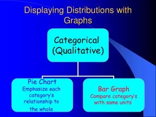
Relative frequency, cumulative frequency, percentiles, and ogives. • Percentile (pth percentile)- The value such that “p” percent of the observations fall at or below it. • Relative frequency - Divide count in each class by total number then multiply by 100 to convert to a percentage. • Cumulative frequency - Add counts in frequency column that fall in or below current class interval.
Cumulative Relative Frequency Divide entries in cumulative frequency column by total number. Ogive pronounced [O-JIVE]. (presidents age) (Percents)(Ogive) (Counts) Relative Cum. Relative Class Frequency Freq. Freq. Cum. Freq. 40-44 2 2/44 = 4.5% 2 2/44 = 4.5% 45-49 7 7/44 = 15.9% 9 9/44 = 20.5% 50-54 13 55-59 12 60-64 7 65-69 3 Total 44
OGIVE: Relative cumulative frequency graph Graph of relative standing of an individual observation.
Various info you can find. • 60th % tile occurs at • age 55 is at about the Bill Clinton = 46 years: • About of all U.S. presidents were the same age as or younger than Bill Clinton or • Bill Clinton was younger than of all U.S. presidents when inaugurated.
Example: Drive Time Professor Moore, who lives a few miles outside a college town, records the time he takes to drive to the college each morning. Here are the times (in minutes) for 42 consecutive weekdays, with the dates in order along the rows:
d. Construct an Ogive for Professor Moore’s Drivetimes.Fill in first 2 rows of relative cum freq. table. We will fill in the rest of the graph together.Note: right most value in range corres. to relative cum. freq. % on ogive. Relative Cumulative Relative Drivetime Frequency FrequencyFrequencyCum.Freq. 6.5-6.91 2.4% 1 2.4% 7.0-7.42 4.8% 3 7.1% 7.5-7.98 19.0% 11 26.2% 8.0-8.411 26.2% 22 52.4% 8.5-9.012 28.6% 34 81.0% 9.1-9.46 14.3% 40 95.2% 9.5-9.91 2.4% 41 97.6% 10.0-10.41 2.4% 42 100%
Remember: begin ogive with a point at height 0% at left endpoint of lowest class interval; last point plotted should be at a point of 100% • 60th percentile occurs at about age 57
Example: Drive Time cont. e. Use your ogive(graph) from b. to estimate the center and 90th percentile for the distribution. • center: about 8.4 How did you find the center? • From graph • Or 2ndSTAT:MATH:median • By hand: 42 observations, the average of the 21st and 22nd observation. (see table) • 90th percentile: approximately 9.4
f. Use your ogive to estimate the percentile corresponding to a drive time of 8.00 minutes. 8.0 is approximately the 26th percentile 100 90 80 70 60 Relative Cumulative Frequency 50 40 30 20 10 0 7.5 8.0 8.5 9.0 9.5 10.0 10.5 7.0 Drive Time (minutes)
Standardizing and Z-Scores All normal curves are the same if we measure in units of size σ about the mean μ as center. Changing to these units is called standardizing. • If x is an observation from a distribution that has mean μ and standard deviation σ, then the standardized value, called the z-scoreof x is:
Standardizing and Z-Scores A z-score tells us how many standard deviationsthe original observationfalls away from the meanand inwhich direction. • Observations larger than the mean are positive. • Observations smaller than the mean are negative.
Standard Normal Distribution • If a variable x has any normal dist. N(μ,σ), • Then the new standardized variable produced has the standard normal distribution. OriginalStandardizeNew x, N(μ,σ) z z, N(0,1)
Standardizing • Standardizing gives a common scale and produces a new variable that has the standard normal distribution.
Exercise 2: Comparing Batting Averages • Three landmarks of baseball achievement are Ty Cobb’s batting average of .420 in 1911, Ted Williams .406 in 1941, and George Brett’s .390 in 1980. • These batting averages cannot be compared directly because the distribution of major league batting averages has changed over the years. • While the mean batting average has been held roughly constant by rule changes and balance between hitting and pitching, the standard deviation has dropped over time.
Here are the facts: Decade Mean Std. Dev 1910’s .266 .0371 1940’s .267 .0326 1970’s .261 .0317 Compute the standardized batting averages for Cobb, Williams, and Brett to compare how far each stood above his peers.
Who was the best among his peers? • Cobb(.420 ); 1910’s (.266,.0371) : z = z = 4.15 • Wiliams(.406 ); 1940’s(.267,.0326): z = 4.26 • Brett(.390 ); 1970’s(.261,.0317): z = 4.07 Williams z-score is the highest. .420 - .266 .0371