Download
1 / 17
170 likes | 449 Vues
Recap…. Kinetic energy and temperature. Thermal & Kinetic Lecture 6 The Maxwell-Boltzmann distribution. LECTURE 6 OVERVIEW. Distributions of velocities and speeds in an ideal gas. Last time…. Free expansion. The ideal gas law. Boltzmann factors.

E N D
Recap…. Kinetic energy and temperature Thermal & Kinetic Lecture 6 The Maxwell-Boltzmann distribution LECTURE 6 OVERVIEW Distributions of velocities and speeds in an ideal gas
Last time…. Free expansion. The ideal gas law. Boltzmann factors.
For a system in thermal equilibrium at a certain temperature, the components are distributed over available energy states to give a total internal energy U. …but what is the probability of finding a particle in a given energy state? The probability of finding a component of the system (eg. an atom) in an energy state e is proportional to the Boltzmann factor: (NB: T is in Kelvin) Boltzmann factors “Available energy is the main object at stake in the struggle for existence and the evolution of the world.” Ludwig Boltzmann “At thermal equilibrium all microscopic constituents of a system have the same average energy” (Grant & Phillips, p. 421) …….now let’s consider the distribution of energy in the system.
Boltzmann’s Law Erratum NB. You will be expected to be able to derive Eqn. 2.21 (i.e. Boltzmann’s law) – see derivation under Section 2.3 in the notes. You have also seen this derivation in the Mathematical Modelling course. Small – though important – typographical error in Eqn. 2.17 – should have: dP = dn’kT
Eg. Diamond is less thermodynamically stable than graphite (can burn diamond in air at ~ 1300 K). Given a few million years diamonds might begin to appear a little more ‘grubby’ then they do now. Why? Boltzmann factors and distributions Yes, but so what? At the start of the derivation (Section 2.3) we said that any force was appropriate – thus, this is a general expression. Assuming conservative force. Boltzmann factors appear everywhere in physics (and chemistry and biology and materials science and…….) Why? Because the expression above underlies the population of energy states and thus controls the rate of a process.
? It is possible to have a time invariant unstable state – can you sketch the potential energy curve associated with this state? Unstable (transient) DE Metastable Stable (ground state) Probability of surmounting barrier proportional to: Stability, metastability and instability Potential energy The hill represents a kinetic barrier. The ball will only surmount the hill when it gains enough energy. (Diamond is metastable with respect to graphite)
The probability of finding a system in a state with energy DE above the ground state is proportional to: E3 E2 E1 Boltzmann factors and probability PROBLEM: You know that electrons in atoms are restricted to certain quantised energy values. The hydrogen atom can exist in its ground state (E1) or in an excited state (E2, E3, E4 etc….). At a temperature T, what is the relative probability of finding the atom in the E3 state as compared to finding it in the E2 state?
You know that electrons in atoms are restricted to certain quantised energy values. The hydrogen atom can exist in its ground state (E1) or in an excited state (E2, E3, E4 etc….). At a temperature T, what is the relative probability of finding the atom in the E3 state as compared to finding it in the E2 state? • exp (E3/kT) • exp (E2/kT) • exp ((-E3+E2)/kT) • exp ((-E2-E3)/kT)
Molecular vibrations and rotations are also quantised. Boltzmann factors and probability ! This is a very important value to memorise as it gives us a ‘handle’ on what processes are likely to occur at room temperature. The value of kT at room temperature (300 K) is 0.025 eV.
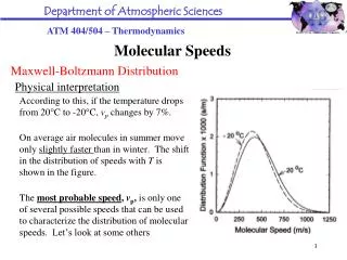
In common with a considerable number of textbooks I use the terms ‘atom’ and ‘molecule’ interchangeably for the constituents of an ideal gas. Consider the distribution of kinetic energies – i.e. the distribution of speeds – when the gas is in thermal equilibrium at temperature T. Speed v is continuously distributedand is independent of a molecule’s position. The distribution of velocities in a gas Let’s now return to the question of molecular speeds in a gas. For the time being we’re concerned only with ideal gases – so: No interactions between molecules Monatomic - no ‘internal energies’ – no vibrations or rotations For an ideal gas the total energy is determined solely by the kinetic energies of the molecules.
vz ? vx What is the kinetic energy of a molecule whose velocity components lie within these ranges? vy ? ..which means that the probability of a molecule occupying a state with this energy is…..? The distribution of velocities in a gas Consider components of velocity vector. Velocity components lie within ranges: vx → vx + dvx vy → vy + dvy vz → vz + dvz ANS: ½ mv2
…which means that the probability of a molecule having this energy is proportional to: • exp (-mv2/2KT) • exp(-mvx/kT) • exp(-mv/kT) • exp(-mv2/kT)
Therefore the probability, f(vx, vy, vz) dvxdvydvz , that a molecule has velocity components within the ranges vx → vx + dvx etc.. obeys the following relation: “OK, but how do we work out what the constant A should be….?” f(vx, vy, vz) exp (-mv2/2kT) …… but v2 = vx2 + vy2 + vz2 constant The distribution of velocities in a gas f(vx, vy, vz) = Aexp (-mvx2/2kT) exp (-mvy2/2kT) exp (-mvz2/2kT)
What is the probability that a molecule has velocity components within the range -∞ to +∞? • 0 • exp(-mv3/kT) • 1 • None of these
? What is the probability that a molecule has velocity components within the range - to +? Hence: In addition, if we’re interested in the probability distribution of only one velocity component (e.g. vx), we integrate over vy and vz: The distribution of velocities in a gas “OK, but how do we work out what the constant A should be….?” ANS:1
We can look up the integral in a table (if required, you’ll be given the values of integrals of this type in the exam) or (better) consult p. 40-6 of the Feynman Lectures, Vol. 1 to see how to do the integration. which means: The distribution of velocities in a gas …and we end up with:
f(vx)dvx FWHM vx 0 Gaussian distributions Expression for f(vx)dvx represents a Gaussian(or normal) distribution where is the standard deviation, (s = FWHM/√(8ln2)) and m is the mean.