Download
1 / 22
370 likes | 1.08k Vues
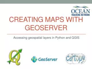
Creating Maps with Geoserver. Accessing geospatial layers in Python and QGIS. What is Geoserver?. Open source solution for sharing geospatial data Access, share, and publish geospatial layers Define layer sources once, access them in many formats. KML. . csv. Shapefiles. Vector Files.

E N D
Creating Maps with Geoserver Accessing geospatial layers in Python and QGIS
What is Geoserver? • Open source solution for sharing geospatial data • Access, share, and publish geospatial layers • Define layer sources once, access them in many formats KML .csv Shapefiles Vector Files GIS Apps Raster Files Geoserver Layers GeoJSON
Geoserver @ OTN • Layers served out of the OTN PostGIS database • A few standard public data products available: • Station deployment information (otn:stations, otn:stations_series) • Public animal release information (otn:animals) • Metadata for projects (otn:otn_resources_metadata_points) • Potential to create private per-project layers for HQP use. • Today: two ways to query the OTN Geoserver • code-based (Python) • GUI-based (QGIS)
Querying Geoserver using Python: • “If you wish to make an apple pie from scratch, you must first invent the universe.” – Carl Sagan • What we’ll need: • Python (2.7 or better) • The following packages: • numpy, matplotlib, geojson, owslib, cartopy • Optionally • A nice Interactive Development Environment to work in. • Spyder (free) • PyCharm (cheap and worth it!)
Accessing Geoserver using owslib • Many services available via Geoserver • Shape and point data – Web Feature Service • Rather under-documented at the moment: • To connect to a Geoserver that is implementing WFS: • from owslib.wfs import WebFeatureService • wfs = WebFeatureService(url, version=“2.0.0”) • OTN Geoserver url = “http://global.oceantrack.org:8080/geoserver/wfs?” • wfs is now a handle to our Geoserver, and we can run queries like: • wfs.contents = a list of all layers served up by Geoserver • wfs.getfeature(typename=[layername], outputFormat=format) • Using the results of getfeature requests, we can build geospatial datasets
Python example: owslib_example.py • Simple script to • connect to Geoserver • grab a layer that defines all stations • generate a printable map • Tools: cartopy, matplotlib, geojson, owslib • Also used: NaturalEarthshapefiles as retrieved by cartopy • naturalearthdata.com
Connecting to Geoserver/ getting layers • # Imports to get the data out of GeoServerfromowslib.wfsimportWebFeatureServiceimportgeojsonimportnumpyasnp# Imports to plot the data onto a mapimportcartopy.crsasccrsimportcartopy.featureas featureimportmatplotlib.pyplotasplt • wfs= WebFeatureService('http://global.oceantrack.org:8080/geoserver/wfs?', version="2.0.0") • # Print the name of every layer available on this Geoserverprint list(wfs.contents) • > [‘discovery_coverage_x_mv’, ‘otn:stations_receivers’, ‘otn:stations’, …] • # Get a list of all stations. Lot of metadata associated with this JSON data.# But for now we're interested in the coordinates.json_response= wfs.getfeature(typename=['otn:stations'], propertyname=None, outputFormat='application/json').read()geom= geojson.loads(json_response)flip_geojson_coordinates(geom) • # geom contains a collection of features, and their default coordinate reference system is a stored property of the collection.print geom['type'], geom['crs'] # check our coordinate reference system> FeatureCollection{u'type': u'EPSG', u'properties': {u'code': u'4326'}}
Geometry object into Cartopy map • ax = plt.axes(projection=ccrs.PlateCarree()) # PlateCarree just simplest map projection for this example • # Get a list of all features.locs= geom.get("features", [])# Each feature has a lot of reference data associated with, as defined in Geoserver.print locs[0]['properties'].keys() • > [u'station_type', u'notes', u'locality', u'collectioncode', u'longitude', u'stationclass', u'depth', u'latitude', u'station_name', u'stationstatus'] • print locs[0]['properties'].values() • > [u'Acoustic', … , u'CapeNorth to St. Paul Island.', u'CBS', -60.33438, u'deployed', 162, 47.06696, u'CBS008', u'active'] • # You can subselect here if you need only some of the stationslons, lats= zip(*[(x["geometry"]["coordinates"][0], x["geometry"]["coordinates"][1]) for x inlocsif x['properties']['collectioncode']==”HFX"]) • # Do some simple buffering of the map edges based on your returned data.plt.axis([min(lons)-1, max(lons)+1, min(lats)-1, max(lats)+1]) • # Plot the lons and lats, transforming them to the axis projectionax.scatter(lons, lats, transform=ccrs.PlateCarree(), edgecolors="k", marker='.’) • ax.stock_img() # fairly nice looking bathymetry provided by Cartopy • # put up some nice looking grid linesgl=ax.gridlines(draw_labels=True)gl.xlabels_top= Falsegl.ylabels_right= False • # Add the land mass coloringsax.add_feature(feature.NaturalEarthFeature('physical', 'land', '10m',edgecolor='face', facecolor=feature.COLORS['land'])) • # You can also define a feature and add it in a separate commandstates_provinces= feature.NaturalEarthFeature('cultural', 'admin_1_states_provinces_lines', scale='50m', facecolor='none')ax.add_feature(states_provinces, edgecolor='gray’) • # There's also a very simple method to call to draw coastlines on your map.ax.coastlines(resolution="10m”) • plt.show()
Geoserver data using GIS tools (QGIS) • Lots of tools available to plot data from Geoserver and combine it with data from other sources • ArcGIS, QGIS, cartodb.com • QGIS is free and open-source, so it will be our example • Download available at: • http://www.qgis.org • Complete manual online at: • http://docs.qgis.org/2.2/en/docs/user_manual/
What we’ll need – using QGIS • Open source tradeoffs: • QGIS is easy to use, but can sometimes be hard to install • NaturalEarth (again, but we’ll get it directly this time) • Grab the NaturalEarthQuickstart pack from naturalearthdata.com • http://kelso.it/x/nequickstart - includes QGIS and ArcMap pre-made projects
QGIS – using NE Quickstart’s .qgs • Open Natural_Earth_quick_start_for_QGIS.qgs • Lots of very nice layers pre-styled for you • Can take it as it is, or choose to hide some of the ones you don’t need by deselecting: • 10m_admin_1_states_provinces • 10m_urban_areas • etc.
Adding our Geoserver to QGIS • Layer - Add WFS Layer • Click New button to add a new source for our WFS layers • Geoserver’s URL a bit different for QGIS: • http://global.oceantrack.org:8080/geoserver/ows?version=1.0.0& • Username/password not required for public layers • Can provide authorization for private layers here
Adding/styling a Geoserver layer • Highlight the layer you want, click Add • The layer appears in your layer list – make sure it’s above the ne_quickstart we added earlier (will be drawn on top) • Double-click to open Layer Properties. Hit Style sub-tab • Change Single Symbol to Categorized • For Column, use ‘collectioncode’ • Hit Classify button • Hit Apply • Stations are grouped and color-coded for you • Further refine station classifications – render certain lines • Can delete all undesired classification groups • Could use rule-based filtering in Style
Tools make everything easier • Now that we have our stations, let’s use some detection data • Layer – Add Delimited Text Layer • Select a Detection Extracts file from the OTN Repository • Since this file has Latitude and Longitude, QGIS recognizes its location information and plots it onto a layer • All associated data from the file is available to use for filtering/styling/summarizing • Detection Extracts not special, any .csv with lat/lon columns can be ingested this way.
QGIS Print Composer • Lock in a certain style and image layout for printing • Define map areas, inset maps, logos, title graphics, legends • When map layers are updated, legends are repopulated and maps redrawn in-place.
Geospatial Queries in QGIS • Objects in QGIS are shapes, so intersections between shapes / buffer zones from point data can be queried • Results of that query can be highlighted, eg: • Global coverage • By intersection b/tbuffer around stationpointsand coastlineshapefile • Add high seas buoysmanually afterward
OTN’s Geoserver – for you to use • Geoserver provides layers with data from the OTN DB • Using Python/QGIS, plot formats are reproducible when data is added to the OTN Database • QGIS easier to get started with, and lets you spend more time playing with your data’s style and formatting. • More useful information / learning tools: • Cartopy: http://scitools.org.uk/cartopy/docs/latest/ • QGIS: http://www.qgistutorials.com/ • OTN GitLab: https://utility.oceantrack.org/gitlab/