Download
1 / 22
220 likes | 249 Vues
Scatterometer winds for mesoscale dynamics. Ad.Stoffelen@knmi.nl Anton Verhoef, Wenming Lin, Marcos Portabella, Patrick Bunn, Jos de Kloe, Jur Vogelzang, Jeroen Verspeek. Overview. Convection Geophysical Model Function departure, cone distance or MLE QC. Convection.

E N D
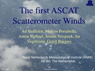
Scatterometer winds for mesoscale dynamics Ad.Stoffelen@knmi.nlAnton Verhoef, Wenming Lin, Marcos Portabella, Patrick Bunn, Jos de Kloe, Jur Vogelzang, Jeroen Verspeek
Overview • Convection • Geophysical Model Function departure, cone distance or MLE • QC
16 February 2014, near 0E, 3N 9:15 9:00 9:30 KNMI MSG rain 9:45 10:00 10:15 ASCAT 9:45 9:45 10:30 ASCAT div ASCAT rot
Convergence and curl structures associated with convective cell • Inflow convergence • Precipitation is associated with wind downburst • Shear zones with curl (+ and -)
KNMI MSG rain 9:00 9:15 9:30 9:45 ASCAT 10:00 10:15 10:30 10:45 ASCAT • Large-scale gust front • Large wind change in 50 minutes over 200-km area 11:00 11:15 11:45 25 February 2014, near 2W, 4N
Developing gust band 25 February 2014, near 2W, 4N 9:00 9:08 ASCAT div 10:00 10:03 10:03 ASCAT div ASCAT rot
MLE – GMF (cone) distance The GMF represents mean conditions on the globe; locally differences occur due to non-nominal conditions: • Sub-WVC wind variability • Rain splash • Rain cloud attenuation and backscatter (Ku band) • Land contamination • Sea ice contamination • Sea structures • . . . • For ASCAT sub-WVC wind variability appears most prominent; most extreme near lows, fronts and convection
TRMMrain MLE: Wind variability Increased wind variability near rain: Downdrafts
ASCAT ambiguities+MLE ECWMF wind+MLE Ambiguity • Ambiguities show streamlines of the flow; can you follow them? • Is ECMWF right? • Do you see consistency in the ASCAT winds and the ASCAT MLEs? • Are there better ASCAT solutions to the ambiguity problem? ASCAT solutions+speed ASCAT solutions+MLE -25, 156
ASCAT ambiguities+MLE ECWMF wind+MLE Use MLE • Denotes flow boundaries • Nowcasting • Ambiguity removal • Proxy for large and short-scale forecast errors • QC to remove un-representative observations in data assimilation ASCAT solutions+speed ASCAT solutions+MLE -8, 95
ASCAT-B and ASCAT-A MLE • ~50 minutes difference only! 33, -137; 18:40/19:30 March 28, 2013
Tropical variability • Dry areas reasonable • NWP models lack air-sea interaction in rainy areas • ASCAT scatterometer does a good job near rain • QuikScat, OSCAT and radiometers are affected by rain droplets • Portabella et al., TGRS, 2011
ASCAT 25 km (selected) winds closer to buoy winds than ECMWF winds in rainy areas (buoy rain data). 14
ASCAT-A ASCAT-B collocation • Global, Dt=50min. • Small spread in NWP due to 50 minutes time difference (smooth wind fields) • Larger spread in ASCAT due to much smaller resolved scales (e.g., convection) ASCAT speeds NWP speed ASCAT-B ASCAT-A
Spatial representation • We evaluate area-mean (WVC) winds in the empirical GMFs • 25-km areal winds are less extreme than 10-minute sustained in situ winds (e.g., from buoys) • So, extreme buoy winds should be higher than extreme scatterometer winds • Extreme global NWP winds should be generally lower due to lacking resolution (over sea)
QC: Which error is acceptable? MLE>+18.6 SDf = 2.31 ms-1 SDf = 1.84 ms-1 SDf = 0.6 ms-1 We can produce winds with SD of buoy-scatterometer difference of 0.6 m/s, but would exclude all high-wind and dynamic air-sea interaction areas The winds that we reject right now in convective tropical areas are noisy (SD=1.84 m/s), but generally not outliers! What metric makes sense for QC trade-off?
12.5 km ASCAT 25 km 18
KNMI HY2A vs ECMWF • NWP ocean calibration (standard for wind processing) • Speed, direction and vector components • Outlier detection • Small scales evolve fast, so when we want to determine (initialize) them in 4D, we will need many observations 1.48 m/s 10.58 deg 1.44 m/s 1.44 m/s
Summary • ASCAT-A and –B tandem are excellent for investigating dynamical aspects of convection • MLE denotes gustiness and wind variability • MLE complements imagery, particularly in case of convection or in pin-pointing extratropical fronts under a heavy cloud deck • MLE could be used in 2DVAR and NWP • Do not throw valuable ASCAT data away, unless you cannot handle it
Triple collocation Data from November 2012 to January 2013 • Errors on scatterometer scale • A and B very similar