Introduction to SPSS (Version 16)
Introduction to SPSS (Version 16). LINDSEY BREWER CSSCR (CENTER FOR SOCIAL SCIENCE COMPUTATION AND RESEARCH) UNIVERSITY OF WASHINGTON September 17, 2009. Topics we will cover today. SPSS at a glance Basic Structure of SPSS Cleaning your data Descriptive Statistics Charts

Introduction to SPSS (Version 16)
E N D
Presentation Transcript
Introduction to SPSS(Version 16) LINDSEY BREWER CSSCR (CENTER FOR SOCIAL SCIENCE COMPUTATION AND RESEARCH) UNIVERSITY OF WASHINGTON September 17, 2009
Topics we will cover today • SPSS at a glance • Basic Structure of SPSS • Cleaning your data • Descriptive Statistics • Charts • Data manipulation • Other Resources
SPSS at a glance • SPSS stands for Statistical Package for the Social Sciences • SPSS was made to be easier to use then other statistical software like S-Plus, R, or SAS. • The newest version of SPSS is SPSS 17.0. Today we will be working on SPSS 16.0.
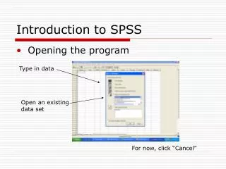
How to open SPSS • Go to START • Click on PROGRAMS • Click on SPSS INC • Click on SPSS 16.0 • The computers in the CSSCR lab typically have SPSS on the desktop. It is a red box that says SPSS on the top.
Opening a data file • Click on FILE OPEN DATA • Click MY COMPUTER LOCAL DISK C:/ • Click PROGRAM FILES SPSS • Click TUTORIAL SAMPLE FILES • Select CATALOG.SAV
Basic structure of SPSS • There are two different windows in SPSS • 1st – Data Editor Window - shows data in two forms • Data view • Variable view • 2nd – Output viewer Window – shows results of data analysis • *You must save the data editor window and output viewer window separately. Make sure to save both if you want to save your changes in data or analysis.*
Data view vs. Variable view • Data view • Rows are cases • Columns are variables • Variable view • Rows define the variables • Name, Type, Width, Decimals, Label, Missing, etc. • Scale – age, weight, income • Nominal – categories that cannot be ranked (ID number) • Ordinal – categories that can be ranked (level of satisfaction)
Cleaning your data – missing data • There are two types of missing values in SPSS: system-missing and user-defined. • System-missing data is assigned by SPSS when a function cannot be performed. • For example, dividing a number by zero. SPSS indicates that a value is system-missing by one period in the data cell.
User-defined missing data are values that the researcher can tell SPSS to recognize as missing. For example, 9999 is a common user-defined missing value. To define a variable’s user-defined missing value… Cleaning your data – missing data • Look at your variables in VARIABLE VIEW • Find the column labeled MISSING • Find the variable that you would like to work with. • Select that variable’s missing cell by clicking on the gray box in the right corner. • click DISCRETE MISSING VALUES • enter 9999 to define this variable’s missing value • A range can also be used if you only want to use half of a scale.
Cleaning your data – missing data cont. When you have missing data in your data set, you can fill in the missing data with surrounding information so it does not affect your analysis. • click TRANSFORM • click REPLACE MISSING VALUES • select the variable with missing values and move it to the right using the arrow • SPSS will rename and create a new variable with your filled in data. • click METHOD to select what type of method you would like SPSS to use when replacing missing values. • click OK and view your new data in data view
Descriptive Statistics • Lets say we are interested in learning more about the number of customer service representatives (service). • Click ANALYZE • Click DESCRIPTIVE STATISTICS • Click FREQUENCIES • Choose service from the list.
Descriptive Statistics continued • Lets learn more about the number of catalogs mailed (mail). • Click ANALYZE • Click DESCRIPTIVE STATISTICS • Click DESCRIPTIVES • Move MAIL over with the arrow • Click OPTIONS – we can choose which statistics we are interested in looking at • We should remember that these descriptive statistics will not always make sense for every variable. For example, we should not be asking for the mean of nominal variables like gender or race.
Graphing Data • Click GRAPH • Click CHART BUILDER • Click HISTOGRAM • Put MEN on the X axis. • Click ELEMENT PROPERTIES. Check the box labeled DISPLAY NORMAL CURVE. This will impose a normal curve onto your graph. You can also change the style of your graph in this element properties window. • You can copy and paste these graphs into word and excel files.
Graphing Continued • There are other ways to make graphs. • Click ANALYZE • Click DESCRIPTIVE STATISTICS • Click FREQUENCIES • Click services • Click CHART • Click BAR CHART • Click PERCENTAGES
By selecting cases, the researcher can select only certain cases for analysis click DATA click SELECT CASES click RANDOM SAMPLE OF CASES select your preferences Data manipulation – select cases
Data manipulation – compute new variable Computing new variables – create a new variable from multiple variables click TRANSFORM click COMPUTE fill in the new target variable TOTALSALES fill in numeric expression = men+women+jewel create an IF statement by clicking on the IF button click INCLUDE IF CASE SATISFIES CONDITION enter condition MAIL>10000 • This new variable TOTALSALES tells us what the total sales are for catalogs which mailed over 10,000 catalogs.
Data manipulation in action! • Try creating another variable for TOTALSALES2 for catalogs which mailed under 10,000 catalogs. • Try comparing the descriptive statistics of TOTALSALES and TOTALSALES2. • What did you find?
Recoding allows a researcher to create a new variable with a different set of parameters click TRANSFORM click RECODE INTO DIFFERENT VARIABLE Data manipulation – recode a variable • move mail over to the right • create a name for the new variable mailcategories • click OLD AND NEW VALUES
click RANGE to create ranges of old values click VALUE to create a new value for that range Data manipulation – recode a variable cont.
Data manipulation in action! • Try recoding another variable on your own. • Try finding the descriptive statistics of your new variable.
Dummy variables is a variable that has a value of either 0 or 1 to show the absence or presence of some categorical effect Data manipulation – create a dummy variable • To create a dummy variable… • click TRANSFORM • click RECODE INTO DIFFERENT VARIABLE • click OLD AND NEW VALUES • click RANGE to create range of old values • click VALUE to set new value to 0 or 1
What we have learned! • SPSS at a glance • Basic Structure of SPSS • Cleaning your data – missing data • Descriptive Statistics – frequencies, descriptive statistics • Charts • Data manipulation – select cases, recoding, dummy variables
Other Resources • There are many resources online to help you learn SPSS (tutorials, blogs, etc.) • CSSCR has a Quicktime SPSS class on its website • CSSCR offers SPSS handouts which are also on its website • CSSCR offers classes on SPSS each quarter – come back for the SPSS Beyond the Basics class!