Download
1 / 79
790 likes | 1.09k Vues
Real-World Evolution of the Yield Curve. Riccardo Rebonato Sukhdeep Mahal Royal Bank of Scotland - QUARC Geneva 2002. The problem. There exist a very large number of models that produce the evolution of the yield curve under a variety of assumptions. Examples :

E N D
Real-World Evolution of the Yield Curve Riccardo Rebonato Sukhdeep Mahal Royal Bank of Scotland - QUARC Geneva 2002
The problem • There exist a very large number of models that produce the evolution of the yield curve under a variety of assumptions. • Examples : • One-factor short-rate models (BDT, BK, HW) • HJM/BGM • Multi-factor short-rate models (LS, HW, RR) • etc.
Why do we need another one? • All these models produce the evolution of the yield curve in the risk-adjusted measure, not in the real-world measure. For risk management purposes I need to evolve the yield curve in the real measure (and, contingent on the future state of the world having been attained, to value instruments in the risk-adjusted measure).
Does it really make a difference? • Consider the case of commodities: a forward-curve in backwardation does not reflect future real-world expectations, but the premium assigned to holding the physical commodity today.
Objection • With commodities cash-and-carry arbitrage does not really work. Perhaps everything is fine with forward rates. • Consider the LMM. The forward rates display a drift upward or downwards depending on the (arbitrary) choice of numeraire. Imagine the effect after 10 years.
Why is there a difference between the two measures? • The forward rates contain an expectation component and a risk premium. • Heath (HJM): ‘The forward rates have nothing to do with expectation of future rates’. A bit too strong. • At very short horizons, it would take an extremely risk-averse utility function to drive an appreciable wedge between expectations in different measures. Over long horizons, the differences can become very large.
Why do I need to evolve the yield curve? • Typical market risk (trading book) applications require to evolve the yield curve over very small steps (1 day, 10 days). • The risk premium is not a big issue. • For other risk-management applications the time horizon can be orders of magnitude longer.
What are these applications? • Counterparty credit risk exposure • Analysis of effectiveness of hedging/trading strategies • A/L (balance sheet) management • Performance analysis and asset allocation choice for investment portfolios
The methodology • Constructing a series of IR paths The goal is to produce future IR paths that incorporate as accurately as possible the information from historical correlated moves of yield curves, collected over a long period of times.
Do we need accurate paths? These simulations must be accurate because they will be used • to make comparison between different asset classes • to gauge risk/reward profiles • to establish reasonable bands of variation for the NII • To test hedging strategies under realistic scenarios (not just the usual rigid shifts up and down of the yield curve)
The usual solution • Do a PCA of the (relative) changes • Retain m eigenvectors • Rescale the eigenvalues • Evolve the yield curve by drawing iid random draws (one for each factor and time step)
Observation 1 • The procedure is valid only if the underlying joint process is a diffusion. I can always orthogonalize a covariance matrix, and work with the eigen-vectors/values, but I will only get back the original process if the original process was a joint diffusion with iid increments to start with.
Observation 2 • By drawing iid random draws that are independent both across factors and serially one is making a very strong assumption about the homoskedaticity and the lack of serial dependence in the data • I shall show that these assumptions are strongly unwarranted
A naïve approach (totally non-parametric) • Collect a large number of synchronous changes in yields, labelled by an index i, i=1,2,…,n. • Draw a uniform variate from U[0,1] • Map the variate to an integer between 1 and n, say, k • Apply the k-th vector of rate changes to the current yield curve • Continue
Comment The approach might be simple, but it is by construction guaranteed to recover as best as possible given the sample size: • all the correct PC (eigenvectors and eigenvalues) • all the correct unconditional marginal distributions for all the yields (all moments). Not every method can deliver this!
Real yield curves just do not look like this! • How can we quantify this lack of ‘plausibility’? • The origin is clearly in the curvature: in real life we observe sharp changes in slope at the very short end, but not as pronounced for longer maturities.
Comments • At the short end the curvature can be very high, both positive and negative - short terms expectations influence the forward rates a lot • At the longer end the distribution of curvatures is much more peaked
What keeps the yield curve smooth? • Assume that, as the yield curve ‘diffuses’, small ‘kinks’ appear • ‘Arbitrageurs’ are enticed to move in with barbell trades, receiving the high yields and paying the low one • This automatically reduces the curvature
Why don’t arbitrageurs do the same at the short end? • At the short end they are afraid that the kink in the curve might reflect expectations about rapidly changing rate expectations (V-shaped recovery of 2001) • At the long end it is more difficult to make an expectation story around the 9-10 year area • The longer the maturity, the fewer the kinks
How can we model this? • Consider a HLH barbell: buying the high yields and selling the low yield is equivalent to introducing springs in the yield curve • This is reflected in a drift term proportional to the local curvature • End effects to be treated separately
How do we choose the spring constants? • We can choose the different spring constants across the yield curve in such a way that the model-produced distribution of curvatures will match some features (eg second moment) of the real-world distribution of curvatures as a function of maturity • So, at the short end the springs are very weak (large curvatures can occur). • At the long end curvatures are strong (curve does not get kinky).
An added bonus • To the extent that what has been added is a drift term, asymptotically I have not affected the covariance matrix • Therefore the new procedure preserves all the positive features of the naïve approach • In particular it still recovers correctly all the eigenvalues and the eigenvectors (PCA) and the unconditional marginal distributions
A Comment Incidentally, this gives an idea of how weak the PCA requirement really is!
More comments • The proposed mechanism introduces (negative) serial correlation in the data points • This effect will be stronger at the long end • This has an impact on the unconditional variance of the various rates. How can we handle this? • Let’s look at real-world data.
Empirical Observation • The variance of short-maturity rates increases more than linearly with time • The variance of long-maturity rates increases less than linearly with time • The cross-over point is around the 2-year maturity
Two simultaneous mechanisms: • The spring-constant mechanism (mean-reversion) makes the unconditional variance grow less than linearly. • The presence of positive serial correlation would make the unconditional variance grow more than linearly. • If this is correct this should be reflected in the serial auto-correlograms: positive serial correlation would make the variance of all rates grow super-linearly, but the strong springs at the long end would reduce this super-linear growth by introducing negative autocorrelation. • Let’s check!