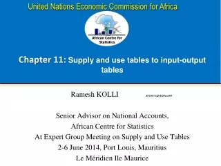
Input-Output Tables
Input-Output Tables. Marc Prud’Homme University of Ottawa Last update: 14/09/12. Introduction.


Input-Output Tables
E N D
Presentation Transcript
Input-Output Tables Marc Prud’Homme University of Ottawa Last update: 14/09/12
Introduction • Applications of I-O family have been published not only in the broader social science fields including but not limited to economics, regional science, international development, but also in the tourism field. • I-O framework is the foundation of System of National Accounts (SNA), which has been used by all the national governments in the world to measure important data such as gross domestic product (GDP), capital formation etc.
History • Dr.Wassily Leontief succeeded in materializing the concept of “Tableau Economique” presented by the French Economist Francois Quesnay, in 1758. • Dr. Leontief published the U.S. Input-Output table of 1919 and 1929, in 1936 (Leontief, 1951), followed by a series of publications, resulting in the 1973 award of the Nobel Prize in Economics "For the development of the input-output method and for its application to important economic problems."
Concept of simple input-output modelling • Let’s assume that we want to learn about our society, and let’s assume that our society consists of three industrial sectors only, namely agriculture, manufacturing and services sectors. • The model is a simplified version of the complex society.
Understanding Intermediate Goods and Final Consumption • Assume that you want to purchase an apple juice in a plastic bottle to quench your thirst. • Here is the first important question. What does the apple juice bottle consist of? • Is it a manufactured product, or an agricultural product? • The plastic bottle is the manufactured product. • The apples however came from the agricultural sector.
Understanding Intermediate Goods and Final Consumption • The manufacturing sector purchased the output –the apples - from the agricultural sector, not to be consumed, but to be used as intermediate goods for producing the final product - the apple juice. • If the manufacturer is the food processing company, they must have bought the empty bottles from another manufacturing sector, thus the manufacturing sector is selling plastic bottles to the other firms within the manufacturing sector.
Understanding Intermediate Goods and Final Consumption • When a sector purchases required input from other sectors, in order to produce their own goods, the former are called “intermediate goods” and this type of transaction is called “inter-industry transactions”. • This is in clear contrast with the purchase of the apple juice bottle for your own consumption. • Your purchase (unless you made the purchase to sell to your friends for profit) is deemed as “final consumption”, and is also considered as “final demand”.
Understanding Intermediate Transactions, Final Demands and Total Output • Imagine now that you are an apple farmer, and that you sell your apples (=output) to two kind of purchasers, only: • The manufacturing sector that makes apple juice. • They purchase your apples (=output) as “intermediate goods” in the inter-industry transactions (agricultural output sold to the manufacturing sector). • As for the remaining apples, you decide to take them to the Farmer’s Market, • People directly purchase them for their own consumption, to satisfy their “final demand”. • Intermediate Goods + Final Demand = Total Output • Apples sold to other industries + Apples sold for final demand = All the apples produced
Understanding Intermediate Transactions, Final Demands and Total Output • Are the following Intermediate goods or final demand? • Tomatoes • Car tires • Hard disks • Hotel rooms
Introduction to basic structure of input-output transaction table • The Input-Output table is displayed in a two-dimensional matrix format, with rows and columns. • Rows show the output for each sector, and columns show the input for each sector. • An example:
Interpretations of a Row in Transaction Table • The agricultural sector’s row runs as follows: • [1 2 1 6 10] • This means that in the course of that year, the agricultural sector’s sales • within the same sector were 1, • its sales to the manufacturing sector were 2 • its sales to the service sector were 1 • its sales to Final Demand were 6, • Total output = 10. • To put the number in equation, (1 + 2 + 1) + 6 = 10 • Intermediate goods + Final Demand = Total Output
Interpretations of a Row in Transaction Table • The agricultural sector’s row runs as follows: • [1 2 1 6 10] • This means that in the course of that year, the agricultural sector’s sales • within the same sector were 1, • its sales to the manufacturing sector were 2 • its sales to the service sector were 1 • its sales to Final Demand were 6, • Total output = 10. • To put the number in equation, (1 + 2 + 1) + 6 = 10 • Intermediate goods + Final Demand = Total Output
Interpretations of a Row in Transaction Table • By looking at the row of the agricultural sector, you can see the destination of this sector’s output. • In this case, a total of 4 agricultural goods provided the industrial sectors with intermediate goods and the total of 6 went to final demands. • This table is called a “transaction table” as it captured actual amount of transactions between sectors. • Each industrial sector may have different methods to record their sales volumes, such as numbers of bushels, cars, barrels, or numbers of visitors, attendees, but in the transaction table, it is more convenient to use common monetary values that reflect the exchange of goods and money. • Thus, we use common units such as US$ million or € million.
Interpretations of a Column in Transaction Table • The agricultural sector’s column is:
Interpretations of a Column in Transaction Table • This can be interpreted as follows (all the ingredients of a recipe): • the internal purchases of the agricultural sector were 1 • its purchases from the manufacturing sector were 1 • its purchases from the service sector were 2 • its purchases from Value Added were 6 • thus making the total agricultural sector’s purchases are 10. • Value Added consists of labour, and capital, etc, which we will examine later. • This column shows something very useful in order to understand the structure of each industrial sector, because the numbers that you see in the column depict all the required input, with the bottom number showing the total input for the sector, in the course of one year. • It is great if you noticed that the total output amount equals the total input amount.
The Leontief Inverse Matrix: This is what I-O is all about! • From the transaction table, we will move step by step towards the Leontief Inverse Matrix, which will enable you to calculate series of multipliers. • Important Concept of “Endogenous versus Exogenous” • First of all, we should learn some concepts related to being inside the model and being outside the model. • “Endogenous” means being inside the model • “Exogenous” means being outside of the model. • With input-output modeling, we will retain the inter-industry transactions parts as endogenous • The Final Demand and Total Output columns are left aside since they are exogenous.
A bit about the matrix stuff: the steps to get at the famous Leontief Inverse matrix • X is total output • Total output consists of intermediate goods (AX; where A < 0 <1), and final demand (Y). • The equation can be expressed as AX + Y = X • Intermediate goods + final demands = total outputs • AX is the portion of Total Output which is traded within the industrial sector as intermediate goods; thus A is greater than 0 but smaller than 1. • When we move the AX to the right side of the equation, the sign before AX changes from plus to minus. • Y = X – AX • Final demands = Total output - Intermediate goods • Y = (I – A)X • Final demands = leftover portion of the Total output used for intermediate goods. • X = (I – A)-1Y • (If an inverse of the portion representing leftover used for Intermediate Goods is multiplied by Final Demand, it would equal Total Output) • Finally:
Introduction to basic structure of input-output transaction table • Transactions Table with Inter-Industry Columns only: • This is a 5 x 3 matrix: a square inter-industry matrix + 1 VA row + total input row.
Standardization process: The Standardized Transaction Matrix • This process is rather simple. You take each required input in each column to be divided by the column total (= Total Input). • For example, the relative input from the value added (=labor, capital, imports and others) to the agricultural sector would be calculated as 6 divided by 10 = 6/10 = 0.6
Creating a standardized A-matrix from transaction table • Now, you select the inter-industry part of the matrix only, in order to get a square matrix (i.e. a matrix in which the number of rows equals the number of columns - in our case, 3 x 3). • This standardized square matrix is called an A-matrix. • It was obtained by standardizing each transaction amount as required input, in terms of total input, and only leaving the part with elements of the inter-industry square matrix.
Creating an Identity (I-) matrix • The I-Matrix is the square matrix which works like 1 (one), as we know from algebra, such as 1 x 2 = 2, 0.5 x 2 = 1, 1 – 0.5 = 0.5. • Although the I-matrix works like 1, it looks different from 1, as it is a matrix. • The I-matrix looks like a square matrix whose elements are all zeros, except for the diagonal elements from top left to bottom right, which has 1s.
Subtracting the A-matrix from an I-matrix • By subtracting an square A-matrix from an square I-Matrix, we will have a (I - A) matrix. • For example, if you look at the first row, first column, the I matrix has 1 and the A matrix has 0.1. • Thus, the first row, first column of the (I – A) matrix will have (1 – 0.1) = 0.9.
Calculating an inverse of the (I – A) matrix to create Leontief inverse matrix Invert using Excel
Using the Leontief Inverse Matrix: Simple Output Multiplier Analyses • Let’s put the Leontief Inverse Matrix into action. • Recall the multiplication rule in matrix algebra that when you have a (n x n) square matrix: it can only be multiplied by a suitable matrix, i.e. one whose number of rows equals n. • Also note that a Leontief Inverse Matrix multiplied by a change in Final Demand yields a change in Total Output. • We can put the combined knowledge into action, as follows: • Matrix algebra (3 x 3) x (3 x1) = (3 x1) • (Leontief Inverse Matrix x Change in Final Demand = Change in Total Output)
Using the Leontief Inverse Matrix: Simple Output Multiplier Analyses • By introducing the concept of incremental change, we can feed the model with the change in final demand, to see how the economy responds with its total output. • The change in final demand is also called a shock, an initial shock, a direct shock, direct effect or direct impact. • Let’s conduct three cases in which we give a positive increase of 1 to each of the three industrial sectors, one by one. • In this case, the final demand column vector (numbers will be shown as a column) would be as follows: Case 1 = Case 2 = Case 3 =
Using the Leontief Inverse Matrix: Simple Output Multiplier Analyses • In Case 1, we assume that the final demand for the agricultural sector’s output is increased by 1 (if you prefer to put some meaning, say $ 1 million, assuming the I-O transaction table was shown in $ million units). • In Case 2, we assume that the final demand for the manufacturing sector’s output is increased by 1 • In Case 3, we assume that the final demand for the services sector’s output is increased by 1. • http://www.youtube.com/watch?v=IRdVU8tyRDU
Using the Leontief Inverse Matrix: Simple Output Multiplier Analyses • Case 1 Exo. shock The economy Response of total output = 1.18 + 0.22 + 0.35 = 1.75 A change in final demand for the agricultural sector of $1m will lead to a change in total output of 1.75. The output multiplier is 1.75 for the Ag sector. The other multipliers are: 2.40 for the manufacturing sector and 1.66 for the services sector. =
Supply-Use Tables (SUT) • The supply and use framework is the part of the national accounts system which focuses on the production and use of goods and services in an economy. • It reflects the activities of industries in which intermediate products and primary inputs (such as labour and capital) are required. • Supply and use tables show where and how goods and services are produced and to which intermediate or final use they flow.
Supply-Use Tables (SUT) • In the supply table, flows of goods and services are valued at basic prices. In the use table, the flows are valued at purchasers’ prices. • In order to attain identities between supply and use, trade and transport margins and taxes less subsidies on products have to be added to the supply table. • A purchaser’s price for a product is the producer’s price plus supplier’s retail and wholesale margins, separately invoiced transport and insurance charges and non-deductible taxes on products payable by the purchaser. • Purchasers’ prices are the prices most relevant for decision-making by buyers.
Supply-Use Tables (SUT) • Value added is recorded at basic prices. It is the net result of output valued at basic prices less intermediate consumption valued at purchasers’ prices. • The use table contains some supplementary information: gross fixed capital formation, stocks of fixed assets and labour inputs by industry. This information is crucial for productivity analysis and may also serve several other types of analyses, e.g. analysis of employment.
Supply-Use Tables (SUT) • GDP is valued at market prices. This aggregate can be derived from the supply and use tables in three different ways: • as output at basic prices by industry minus the sum of intermediate consumption at purchasers’ prices by industry plus net taxes on products (production approach); • as sum of the various components of value added at basic prices by industry plus net taxes on products (income approach); • as sum of final use categories minus imports: exports – imports + final consumption expenditure + gross capital formation (expenditure approach).