Download
1 / 55
550 likes | 806 Vues
Seismic Analysis of Some Geotechnical Problems – Pseudo-dynamic Approach . Dr. Priyanka Ghosh Assistant Professor Dept. of Civil Engineering Indian Institute of Technology, Kanpur INDIA. Organisation. Introduction to Pseudo-dynamic Approach and Upper Bound Limit Analysis

E N D
Seismic Analysis of Some Geotechnical Problems – Pseudo-dynamic Approach Dr. Priyanka Ghosh Assistant Professor Dept. of Civil Engineering Indian Institute of Technology, Kanpur INDIA
Introduction to Pseudo-dynamic Approachand Upper Bound Limit Analysis • Seismic Bearing Capacity of Strip Footing using Upper Bound Limit Analysis • Seismic Vertical Uplift Capacity of Horizontal Strip Anchorsusing Upper Bound Limit Analysis • Seismic Active Earth Pressure Behind Non-vertical RetainingWall using Limit Equilibrium Method • Seismic Active Earth Pressure on Walls with Bilinear Backface using Limit Equilibrium Method • Seismic Passive Earth Pressure Behind Non-vertical RetainingWall using Limit Equilibrium Method • Conclusions
Introduction to Pseudo-dynamic Approach and Upper Bound Limit Analysis
For a Sinusoidal Base Shaking, the Acceleration at any Depth z below the Ground Surface and Time t
Mass of the Shaded Element m(z) and Total Weight of the Failure WedgeW Total Horizontal Seismic Inertia ForceQh(t) Where, l = wavelength of the shear wave = TVs
Total Vertical Seismic Inertia ForceQv(t) Where, h = wavelength of the primary wave = TVp
Theorem: If a compatible mechanism of plastic deformation , , is assumed, which satisfies the condition = 0 on the displacement boundary Su; then the loads Ti, Fi determined by equating the rate at which the external forces do work to the rate of internal dissipation of energy will be either higher or equal to the actual limit load. Upper Bound Limit Analysis
Equation = displacement rate = plastic strain rate compatible with displacement rate = stress tensor associated with plastic strain rate Ti= external force on the surface S Fi= body forces in a body of volume V
Seismic Bearing Capacity of Strip Footing using Upper Bound Limit Analysis Acta Geotechnica (Springer Pub.), 2008, Vol. 3, No. 2, pp 115-123.
b Pu xPu ah = faahg Footing B D A b a Qv1 Qv2 U21 Qh1 z Qh2 U2 f W1 f W2 Collapse mechanism and velocity hodograph z f U1 Acta Geotechnica (Springer Pub.), 2008, Vol. 3, No. 2, pp 115-123. z dz dz ah = ahg C Vs, Vp (a) U2 U21 (b) (a + b) U1
Variation of NE with ah and av for different values of with H/l = 0.3, H/h = 0.16 for (a) fa = 1.0, (b) fa = 1.2 Acta Geotechnica (Springer Pub.), 2008, Vol. 3, No. 2, pp 115-123.
fa = 1.0 fa = 1.2 fa = 1.4 fa = 1.6 fa = 1.8 fa = 2.0 Effect of soil amplification on NE for different values of ah with = 30o, av = 0.5ah, H/l = 0.3, H/h = 0.16 Acta Geotechnica (Springer Pub.), 2008, Vol. 3, No. 2, pp 115-123. NgE ah
Comparison of NE with fa = 1.0, av = 0.0, H/l = 0.3 and H/h = 0.16 for (a) = 30o, (b) = 40o Acta Geotechnica (Springer Pub.), 2008, Vol. 3, No. 2, pp 115-123.
Seismic Vertical Uplift Capacity of Horizontal Strip Anchors using Upper Bound Limit Analysis Computers and Geotechnics (Elsevier Pub.), 2009, Vol. 36, No. 1-2, pp 342-351.
Failure mechanism and associated forces Computers and Geotechnics (Elsevier Pub.), 2009, Vol. 36, No. 1-2, pp 342-351.
Variation of fE with ah for different values of fa, e and av with = 20o, H/l = 0.3 and H/h = 0.16 Computers and Geotechnics (Elsevier Pub.), 2009, Vol. 36, No. 1-2, pp 342-351.
fa = 1.0 (upper most) 1.2 1.4 1.6 1.8 2.0 (lower most) Effect of soil amplification on fE for different values of ah with = 30o, av = 0.5ah, e = 3.0, H/l = 0.3 and H/h = 0.16 Computers and Geotechnics (Elsevier Pub.), 2009, Vol. 36, No. 1-2, pp 342-351. fgE ah Fig. 5. Effect of soil amplification on fE for different values of ah with = 30o, av = 0.5ah, e = 3.0, H/l = 0.3 and H/h = 0.16.
av/ah = 0.00 (upper most) 0.25 0.50 0.75 1.00 (lower most) Effect of av on fE for different values of ah with = 30o, fa = 1.4, e = 3.0, H/l = 0.3 and H/h = 0.16 Computers and Geotechnics (Elsevier Pub.), 2009, Vol. 36, No. 1-2, pp 342-351. fgE ah Fig. 6. Effect of av on fE for different values of ah with = 30o, fa = 1.4, e = 3.0, H/l = 0.3 and H/h = 0.16.
Geometry of the failure patterns for different values of f with fa = 1.4, e = 3.0, av = 0.5ah, H/l = 0.3 and H/h = 0.16 Computers and Geotechnics (Elsevier Pub.), 2009, Vol. 36, No. 1-2, pp 342-351.
Comparison of fgE for fa = 1.0, av = 0.0, e = 3.0, H/l = 0.3 and H/h = 0.16 Computers and Geotechnics (Elsevier Pub.), 2009, Vol. 36, No. 1-2, pp 342-351.
Seismic Active Earth Pressure Behind Non-vertical Retaining Wall using Limit Equilibrium Method Canadian Geotechnical Journal,2008, Vol. 45, No. 1, pp 117-123.
Failure mechanism and associated forces Canadian Geotechnical Journal,2008, Vol. 45, No. 1, pp 117-123.
q = 10o 5o 0o -5o -10o (lower most) q = 10o 5o 0o -5o -10o (lower most) q = 10o 5o 0o -5o -10o (lower most) Kae Kae Kae Variation of Kae with ah for f = 30o, av = 0.5ah, H/l = 0.3 and H/h = 0.16 (a) fa = 1.0, (b) fa = 1.4 d = f d = 0.5f d = 0.0 Canadian Geotechnical Journal,2008, Vol. 45, No. 1, pp 117-123. ah ah ah (a) q = 10o 5o 0o -5o -10o (lower most) q = 10o 5o 0o -5o -10o (lower most) q = 10o 5o 0o -5o -10o (lower most) Kae Kae Kae d = f d = 0.5f d = 0.0 ah ah ah (b) Fig. 2. Variation of active pressure coefficient Kae with ah for f = 30o, av = 0.5ah, H/l = 0.3 and H/h = 0.16 (a) fa = 1.0, (b) fa = 1.4.
fa = 1.0 fa = 1.2 fa = 1.4 fa = 1.6 fa = 1.8 Normalized seismic active earth pressure distribution for different values of fa (f = 30o, d = 0.5f, q = 10o, ah = 0.2, av = 0.5ah, H/l = 0.3, H/h = 0.16) z/H Canadian Geotechnical Journal,2008, Vol. 45, No. 1, pp 117-123. pae/gH Fig. 3. Normalized seismic active earth pressure distribution for different values of fa (f = 30o, d = 0.5f, q = 10o, ah = 0.2, av = 0.5ah, H/l = 0.3, H/h = 0.16).
f = 20o f = 30o f = 40o f = 50o Normalized seismic active earth pressure distribution for different values of f (d = 0.5f, q = 10o, ah = 0.2, av = 0.5ah, H/l = 0.3, H/h = 0.16, fa = 1.4) Canadian Geotechnical Journal,2008, Vol. 45, No. 1, pp 117-123. z/H pae/gH Fig. 4. Normalized seismic active earth pressure distribution for different values of f (d = 0.5f, q = 10o, ah = 0.2, av = 0.5ah, H/l = 0.3, H/h = 0.16, fa = 1.4).
q = -15o q = -10o q = -5o q = 0o q = 5o q = 10o Normalized seismic active earth pressure distribution for different values of q (f = 30o, d = 0.5f, ah = 0.2, av = 0.5ah, H/l = 0.3, H/h = 0.16, fa = 1.4) q = 15o Canadian Geotechnical Journal,2008, Vol. 45, No. 1, pp 117-123. z/H pae/gH Fig. 5. Normalized seismic active earth pressure distribution for different values of q (f = 30o, d = 0.5f, ah = 0.2, av = 0.5ah, H/l = 0.3, H/h = 0.16, fa = 1.4)
d = 0 d = 0.5f d = f Normalized seismic active earth pressure distribution for different values of f and d (q = 10o, ah = 0.2, av = 0.5ah, H/l = 0.3, H/h = 0.16, fa = 1.4) Canadian Geotechnical Journal,2008, Vol. 45, No. 1, pp 117-123. f = 20o f = 30o z/H pae/gH Fig. 6. Normalized seismic active earth pressure distribution for different values of f and d (q = 10o, ah = 0.2, av = 0.5ah, H/l = 0.3, H/h = 0.16, fa = 1.4)
Geometry of the failure patterns for different values of ah with fa = 1.4, q = 10o, d = 0.5f, av = 0.5ah, H/l = 0.3 and H/h = 0.16 Canadian Geotechnical Journal,2008, Vol. 45, No. 1, pp 117-123.
Comparison of Kae for av = 0.5ah, H/l = 0.3, H/h = 0.16 and fa = 1.0 Canadian Geotechnical Journal,2008, Vol. 45, No. 1, pp 117-123.
Seismic Active Earth Pressure on Walls with Bilinear Backface using Limit Equilibrium Method Computers and Geotechnics (Elsevier Pub.), (In press).
Failure mechanism and associated forces Computers and Geotechnics (Elsevier Pub.), (In press).
θ1 = 90 (upper most) 75 60 45 θ1 = 90 (upper most) 75 60 45 θ1 = 90 (upper most) 75 60 45 δ1 = δ2= 0.5f δ1 = δ2= f δ1 = δ2= 0 θ2 = 120 (upper most) 110 100 90 θ2 = 120 (upper most) 110 100 90 θ2 = 120 (upper most) 110 100 90 δ1 = δ2= 0.5f δ1 = δ2 = f δ1 = δ2= 0 Variation of active pressure coefficients Kae1 and Kae2 with ahfor f = 30˚, H1/H = 1/3, av = 0.5ah, fa = 1.4, H/TVs= 0.3 and H/TVp= 0.16: (a) θ2=100˚ (b) θ1= 75˚ Computers and Geotechnics (Elsevier Pub.), (In press).
Variation of Kae1 and Kae2 for different combinations of q1 and q2 with f= 30˚, d1 = d2 = 0.5f, H1/H = 1/3, av = 0.5ah, fa = 1.4, H/TVs= 0.3 and H/TVp= 0.16 (a) Kae1(b) Kae2 Computers and Geotechnics (Elsevier Pub.), (In press).
Normalized pae distribution for different fa (f= 30˚, d1 = d2= 0.5f, θ1 = 75˚, θ2= 100˚, H1/H =1/3, ah= 0.2, av= 0.5ah, H/TVs = 0.3 and H/TVp = 0.16) Computers and Geotechnics (Elsevier Pub.), (In press).
Normalized pae distribution for different f(d1 = d2= 0.5f, θ1 = 75˚, θ2= 100˚, H1/H =1/3, fa= 1.4, ah= 0.2, av= 0.5ah, H/TVs = 0.3 and H/TVp = 0.16) Computers and Geotechnics (Elsevier Pub.), (In press).
Normalized pae distribution for different θ1and θ2(f = 30o, d1 = d2= 0.5f, H1/H =1/3, fa= 1.4, ah= 0.2, av= 0.5ah, H/TVs = 0.3 and H/TVp = 0.16) Computers and Geotechnics (Elsevier Pub.), (In press).
f = 20° f= 30° Normalized pae distribution for different wall friction and f(θ1 = 75˚, θ2= 100˚, H1/H =1/3, fa= 1.4, ah= 0.2, av= 0.5ah, H/TVs = 0.3 and H/TVp = 0.16) Computers and Geotechnics (Elsevier Pub.), (In press).
Comparison of Kae1 and Kae2 for H1/H = 1/2, = 36˚, d1 = d2 = 18˚, θ1 = 75˚, θ2 = 105˚, v = 0.5h and fa=1.0 Computers and Geotechnics (Elsevier Pub.), (In press).
Seismic Passive Earth Pressure Behind Non-vertical Retaining Wall using Limit Equilibrium Method Geotechnical and Geological Engg. Journal (Springer Pub.),2007, Vol. 25, No. 6, pp 693-703.
Failure mechanism and associated forces Geotechnical and Geological Engg. Journal (Springer Pub.),2007, Vol. 25, No. 6, pp 693-703.
q = -10o -5o 0o 5o 10o (lower most) q = -10o -5o 0o 5o 10o (lower most) q = -10o -5o 0o 5o 10o (lower most) Kpe Kpe Kpe d = 0.0 d = 0.5f d = f ah ah ah Variation of passive pressure coefficient Kpe with ah for f = 30o, av = 0.5ah, H/l = 0.3 and H/h = 0.16 Geotechnical and Geological Engg. Journal (Springer Pub.),2007, Vol. 25, No. 6, pp 693-703.
f = 20o f = 30o f = 40o f = 50o z/H ppe/gH Normalized ppe distribution for different values of f (d = 0.5f, q = 10o, ah = 0.2, av = 0.5ah, H/l = 0.3, H/h = 0.16) Geotechnical and Geological Engg. Journal (Springer Pub.),2007, Vol. 25, No. 6, pp 693-703.
q = -15o q = -10o q = -5o q = 0o q = 5o q = 10o q = 15o z/H ppe/gH Normalized ppe distribution for different values of q (f = 30o, d = 0.5f, ah = 0.2, av = 0.5ah, H/l = 0.3, H/h = 0.16) Geotechnical and Geological Engg. Journal (Springer Pub.),2007, Vol. 25, No. 6, pp 693-703.
d = 0 d = 0.25f d = 0.5f d = 0.75f d = f z/H ppe/gH Normalized ppe distribution for different values of d (f = 30o, q = 10o, ah = 0.2, av = 0.5ah, H/l = 0.3, H/h = 0.16) Geotechnical and Geological Engg. Journal (Springer Pub.),2007, Vol. 25, No. 6, pp 693-703.
Comparison of Kpe for d = 0.5f, q = 0o, av = 0.0, H/l = 0.3 and H/h = 0.16 Geotechnical and Geological Engg. Journal (Springer Pub.),2007, Vol. 25, No. 6, pp 693-703.
Comparison of Kpe for d = 0.5f, q = 10o, av = 0.5ah, H/l = 0.3 and H/h = 0.16 Geotechnical and Geological Engg. Journal (Springer Pub.),2007, Vol. 25, No. 6, pp 693-703.
Strip Footing • The magnitude of NgE decreases with increase in soil amplification, shear and primary wave velocities, which can not be predicted by the existing pseudo-static approach • In the upper-bound solution, for higher values of f, a significant increase in NgE was observed at lower value of ah Acta Geotechnica (Springer Pub.), 2008, Vol. 3, No. 2, pp 115-123.