Download
1 / 34
340 likes | 553 Vues
Graphs of Sine and Cosine Functions. 4.5. Objective: SWBAT graph sine and cosine curves and identify the transformations. What You Should Learn. Sketch the graphs of basic sine and cosine functions Use amplitude and period to help sketch the graphs of sine and cosine functions

E N D
Graphs of Sine and Cosine Functions • 4.5 • Objective: • SWBAT graph sine and cosine curves and identify the transformations
What You Should Learn • Sketch the graphs of basic sine and cosine functions • Use amplitude and period to help sketch the graphs of sine and cosine functions • Sketch translations of graphs of sine and cosine functions • Use sine and cosine functions to model real-life data
Basic Sine and Cosine Curves • Here you will study techniques for sketching the graphs of the sine and cosine functions. The graph of the sine function is a sine curve. • In Figure 4.43, the black portion of the graph represents one period of the function and is called one cycle of the sine curve. • The gray portion of the graph indicates that the basic sine wave repeats indefinitely to the right and left. • Figure 4.43
Basic Sine and Cosine Curves • The graph of the cosine function is shown in Figure 4.44. • Figure 4.44
Basic Sine and Cosine Curves • The domain of the sine and cosine functions is the set of all real numbers. The range of each function is the interval [–1, 1] • and each function has a period 2.
Basic Sine and Cosine Curves • Do you see how this information is consistent with the basic graphs shown in Figures 4.43 and 4.44? • Figure 4.43 • Figure 4.44
Basic Sine and Cosine Curves • To sketch the graphs of the basic sine and cosine functions by hand, it helps to note five key points in one period of each graph: the intercepts, the maximum points, and the minimum points. • The table below lists the five key points on the graphs of • y = sin x and y = cos x.
Basic Sine and Cosine Curves • Note in Figures 4.43 and 4.44 that the sine curve is symmetric with respect to the origin, whereas the cosine curve is symmetric with respect to the y-axis. • These properties of symmetry follow from the fact that the sine function is odd whereas the cosine function is even.
Basic Sine and Cosine Curves • The basic characteristics of the parent sine function and parent cosine function are listed below
Example 1 – Library of Parent Functions: f(x) = sin x • Sketch the graph of g(x) = 2 sin x by hand on the interval[–, 4]. • Solution: • Note that g(x) = 2 sin x = 2(sin x) indicates that the y-values of the key points will have twice the magnitude of those on the graph of f(x) = sin x. • Divide the period 2 into four equal parts to get the key points
Example 1 – Solution • cont’d • By connecting these key points with a smooth curve and extending the curve in both directions over the interval [–, 4], you obtain the graph shown in Figure 4.45. • Figure 4.45
Amplitude and Period of Sine and Cosine Curves • Let us discuss the graphic effect of each of the constants a, b, c,and d in equations of the forms • y = d + a sin(bx – c) and y = d + a cos(bx – c). • The constant factor a in y = a sin x acts as a scaling factor—a vertical stretch or vertical shrink of the basic sine curve. • When |a| >1, the basic sine curve is stretched, and when |a| < 1, the basic sine curve is shrunk.
Amplitude and Period of Sine and Cosine Curves • The result is that the graph of y = a sin x ranges between –a and a instead of between –1 and 1. The absolute value of a is the amplitude of the function y = a sin x. • The range of the function y = a sin x for a > 0 is –aya.
Example 2 – Scaling: Vertical Shrinking and Stretching • On the same set of coordinate axes, sketch the graph of each function by hand. • a.b.y = 3 cos x • Solution: • a. Because the amplitude of is , the maximum value is and the minimum value is – . • Divide one cycle, 0 x 2, into four equal parts to get the key points
Example 2 – Solution • cont’d • b. A similar analysis shows that the amplitude of y = 3 cos x is 3, and the key points are
Example 2 – Solution • cont’d • The graphs of these two functions are shown in Figure 4.46. • Notice that the graph of • is a vertical shrink of the graph of y = cos x and the graph of • y = 3 cos x • is a vertical stretch of the graph of y = cos x. • Figure 4.46
Amplitude and Period of Sine and Cosine Curves • The graph of y = –f(x) is a reflection in the x-axis of the graph of y = f(x). • For instance, the graph of y = –3cos x is a reflection of the graph of y = 3cos x,as shown in Figure 4.47. • Figure 4.47
Amplitude and Period of Sine and Cosine Curves • Next, consider the effect of the positive real number b on the graphs of y = a sin bx and y = a cos bx. • Because y = a sin x completes one cycle from x = 0 to x = 2,it follows that y = a sin bx completes one cycle from x = 0 to x = 2b.
Amplitude and Period of Sine and Cosine Curves • Note that when 0 < b < 1, the period of y = a sin bx is greater than 2 and represents a horizontal stretching of the graph of y = a sin x. • Similarly, when b > 1, the period of y = a sin bx is less than 2 and represents a horizontal shrinking of the graph of y = a sin x. When b is negative, the identities • sin(–x) = –sin x andcos(–x) = cos x • are used to rewrite the function.
Translations of Sine and Cosine Curves • The constant c in the general equations • y = a sin(bx – c)and y = a cos(bx – c) • creates horizontal translations (shifts) of the basic sine and cosine curves. • Comparing y = a sin bx with y = a sin(bx – c), you find that the graph of y = a sin(bx –c) completes one cycle from bx – c =0 to bx – c =2.By solving for x, you can find the interval for one cycle to be
Translations of Sine and Cosine Curves • This implies that the period of y = a sin(bx – c)is 2b, and the graph of y = a sin bx is shifted by an amount cb. The number cb is the phase shift.
Example 4 – Horizontal Translation • Analyze the graph of • Solution: • The amplitude is and the period is 2.By solving the equations • and • you see that the interval • corresponds to one cycle of the graph.
Example 4 – Solution • cont’d • Dividing this interval into four equal parts produces the following key points.
Mathematical Modeling • Sine and cosine functions can be used to model many real-life situations, including electric currents, musical tones, radio waves, tides, and weather patterns.
Example 8 – Finding a Trigonometric Model • Throughout the day, the depth of the water at the end of a dock varies with the tides. The table shows the depths (in feet) at various times during the morning.
Example 8 – Finding a Trigonometric Model • cont’d • a. Use a trigonometric function to model the data. Let t be the time, with t = 0 corresponding to midnight. • b. A boat needs at least 10 feet of water to moor at the dock. During what times in the evening can it safely dock? • Solution: • a. Begin by graphing the data, as shown in Figure 4.53. You can use either a sine or cosine model. Suppose you use a cosine model of the form • y = a cos(bt – c) + d. • Figure 4.53c
Example 8 – Solution • cont’d • The difference between the maximum height and minimum height of the graph is twice the amplitude of the function. • So, the amplitude is • a = [(maximum depth) – (minimum depth)] • = (11.3 – 0.1) • = 5.6.
Example 8 – Solution • cont’d • The cosine function completes one half of a cycle between the times at which the maximum and minimum depths occur. So, the period p is • p = 2[(time of min. depth) – (time of max. depth)] • = 2(10 – 4) • = 12 • which implies that b = 2p 0.524.
Example 8 – Solution • cont’d • Because high tide occurs 4 hours after midnight, consider the left endpoint to be cb =4, so c 2.094. • Moreover, because the average depth is • (11.3 + 0.1) = 5.7 • it follows that d = 5.7. So, you can model the depth with the function • y = 5.6 cos(0.524t – 2.094) + 5.7.
Example 8 – Solution • cont’d • b. Using a graphing utility, graph the model with the line • y = 10. • Using the intersect feature, you can determine that the depth is at least 10 feet between 2:42 P.M. (t 14.7) and 5:18 P.M. (t 17.3), as shown in Figure 4.54. • Figure 4.54