Basic Matlab Tools for Control Calculations: Review & Applications
Explore basic Matlab tools for control system calculations. Enter and clear variables, use functions for roots, transfer functions, simulations, and plotting in Matlab.

Basic Matlab Tools for Control Calculations: Review & Applications
E N D
Presentation Transcript
BAE 3023 Basic tools in Matlab A review of some of the basic tools for controls calculations
Matlab variable entry BAE 3023 • Set variables a=3 b=[3,4,7] row vector c=[3; 4; 7] column vector d=[1,2;3,4] matrix • Show variables who whos • Clear variables clear clear x • Set iterated list e=1:0.2:10 (start : increment : end) • Get Help help help lsim “for help on lsim” • use windows help function
Matlab calculations BAE 3023 • Matlab offers basic mathematical calculation tools that may be used for calculations in control systems. • Summary: • Entry of polynomials as a row vector • For the polynomial: den=[1,1,4] Num=[1] • Roots of a polynomial • For the polynomial: den=[1,1,4] roots(den) • Definition of a transfer function • For the above variables num,den s = tf(num,den) • Calculations involving complex numbers a = 1.1 + 2.7i r = a^2 + a + 4
Matlab simulation BAE 3023 • Simulation of response of a system described by transfer functions • Step input • For the polynomial: den=[1,1,4] num=[1] s = tf(num,den) step(s) Plot will result • Impulse input (as above except:) impulse(s) • General function input (assume the above polynomial) t = 0 : 0.1 : 100; “sets time vector with start : increment : end” u = cos(t); “sets the input function to u for the given time vector” lsim(s,u,t) “outputs a plot of the response over the set time” • u may be any function. Matlab provides generic functions ie. sin, cos, square, triangle, etc.
Matlab plotting BAE 3023 • Simple plotting • Simple x/y plot x=0:1:20 y=sin(x) plot(x,y) • Set line /point type plot(x,y,’c+’) “cyan “+” points “ plot(x,y,’r+’,x,y,’b-’) “red points and blue line” • Set Titles and labels Labels xlabel(‘X-axis’) ylabel(‘Y-Axis’) title(‘Title’)