Sampling Distribution Models
This content explores sampling distribution models in the context of speeding rates on I-10 and voting behavior on Proposition 2. Using statistical methods, we evaluate the proportion of speeders among 50 cars, establishing that it fits a normal distribution with a mean of 0.8 and a standard deviation of 0.057. Additionally, we analyze a random sample of 100 voters, estimating the likelihood of a deadlock based on a proportion of 51%. Through the lens of the Central Limit Theorem, we assert that as sample size increases, distributions approach normality, establishing a framework for interpreting sampled data.

Sampling Distribution Models
E N D
Presentation Transcript
Sampling Distribution Models February 2012
Drawing Normal Models • For cars on I-10 between Kerrville and Junction, it is estimated that 80% are speeding. What proportion of speeders would we expect to see if we counted 50 cars? • Think: Does this fit the normal model? • 10% condition: 50 cars is less than 10% of the cars on the road. • Success/Failure: At least 10 failures and 10 successes? • np = .8(50) = 40 • nq = .2(50) = 10 • It fits the normal model.
Drawing Normal Models • The sampling model for proportion of speeders is normal with mean of 0.8 and standard deviation of • The model for , the sample proportion is N(0.8, 0.057) • Per the 68-95-99.7 model, we would expect 68% of the proportions to be within 1 σ, the interval (.743, .857) • We would expect 95% of the proportions to be within 2 σ, the interval (.686, .914) • An 99.7% within 3 σ: (.629, .971).
Drawing Normal Models • We don’t know it yet, but 51% of voters are planning to vote “Yes” on Proposition 2. We poll a random sample of 100 voters. What is the probability our sample will be opposed or deadlocked? • Does it meet normal criteria? • 10% rule? Check. There are more than 1000 voters. • Success/Failure: Check. 51/49. • What is the distribution for our proportion? • μ = 0.51 • σ = √(.51)(.49)/100 = 0.050. • Therefore, our distribution is N(0.51, 0.05).
Drawing Normal Models • Restating our original question, we want to know the probability of deadlock or voting against. • Since p-hat is N(0.51, 0.05), our critical value is .5. The z-score for .5 is • Therefore P(z<-.20) = .4207. • There is a 42% chance that our sample will not vote in favor of the proposition. • That is not terrific. If the true parameter p is close to .5, then we would need a larger sample to predict the outcome more accurately.
Sampling Distribution for means • If we have a population that has a distribution where mean and variance are defined, then we know that the sample means from that distribution will approach normality as the sample size increases. This is a conclusion of the Central Limit Theorem (check the book for the details). • Conditions: These conditions must be met if we are going to use the Central Limit Theorem. • Randomness: The sample must be selected randomly. • Independence: The individuals must be mutually independent. • 10% condition: Sample size < 10% of the total population. • Large Enough Sample: For symmetric and uni-modal distributions, the sample does not need to be that big. For highly skewed distributions, a large sample is more likely to give good results. At this stage in the game, if n ≥ 30, you can be pretty confident the sample is large enough.
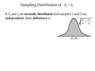
Sampling Distribution for means • If all conditions are met, then we can state that our sampling distribution has a normal model. • If Y is a random variable with known mean (μY) and std. dev. (σY), then Y is a normal random variable. Y ~ N(μY, σY/√n) • The mean of a sample has less variability than individual values, so the standard deviation is divided by the square root of the sample size. • How would we apply this to a real-life situation? • It is know that the mean SAT verbal score is 500 with σ= 100. A sample of 100 AP Statistics students is taken. What would the expected distribution of the mean score be?
Sampling Distribution for means • Known μ = 500 with and σ= 100. Sample size is 100 AP Students. Does it meet the randomness, independence and large enough conditions? • Randomness? NO. These are AP students. We cannot go forward. • Let’s change our sample to just 100 students. That would take care of randomness. How about independence? • We’d have to assume that they were drawn from the entire population. Every student should have an equal chance of being selected. This seems reasonable. And this is far less than 10% of the total population. • Large enough sample? Sure. • Since all three conditions are met, our sample mean, Y ~N(500, 10) • 68%: (490,510); 95%: (480,520); 99.7%: (470,530).
Sampling Distribution for means • Looking to the future: Let’s suppose that we did take a sample of 100 AP students and their average SAT score was 513. • Is that an unusual value? No. The z-score is 1.3. That is well within the expected range of values. What this tells us is that it is possible that the AP students test scores might not be different than all students. It would require additional tests to distinguish between AP and everyone.
Caveats For Sample Distributions • Don’t confuse the distribution of the sample with the sampling distribution. • Beware of dependent observations. One of the assumptions when we assume normality is that of independence. Dependence equals non-random samples. • Beware small samples from skewed populations. Do not assume that your sample is from a unimodal, symmetric population. A sample with a small “n” from a skewed population will likely violate the Central Limit Theorem (CLT). • Homework/Classwork: Problems 2, 4, 5, 9 on page 428.
Application Problems • Suppose weight for adults is normally distributed with μ =175 lb and σ = 25 lb. An elevator has a weight limit of 10 people or 2000 lbs. What is the probability that 10 people getting on the elevator would overload it? • Response to an AP prompt: • Think: Check all my conditions. • Random? Independent? 10%? Large enough? (Assume yes on all) • Show: Tell me that you checked the conditions and that they are OK and then answer the problem. • What is the sampling distribution? How did you calculate it? • Draw a picture of the distribution. Identify the critical value of the sample statistic (in this case the sample mean) and determine the probability of exceeding.
Standard Error • We do not usually know the parameters of a distribution. We estimate the parameters with statistics, so sample mean estimates population mean and sample standard deviation estimates population standard deviation. • When we have to estimate the standard deviation of a sampling distribution, we calculate the standard error. • Standard error for proportion: • Standard error for mean: • We will use the standard error quite frequently. It will come into play when we don’t know p or μ.

