SAMPLING DISTRIBUTION

1. SAMPLING DISTRIBUTION

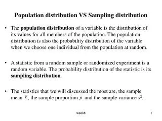
2. Introduction • In real life calculating parameters of populations is usually impossible because populations are very large. • Rather than investigating the whole population, we take a sample, calculate a statistic related to the parameter of interest, and make an inference. • The sampling distribution of the statistic is the tool that tells us how close is the statistic to the parameter.

3. x 1 2 3 4 5 6 p(x) 1/6 1/6 1/6 1/6 1/6 1/6 Sampling Distribution of the Mean • An example • A die is thrown infinitely many times. Let X represent the number of spots showing on any throw. • The probability distribution of X is E(X) = 1(1/6) + 2(1/6) + 3(1/6)+ ………………….= 3.5 V(X) = (1-3.5)2(1/6) + (2-3.5)2(1/6) + …………. …= 2.92

4. Throwing a die twice – sample mean • Suppose we want to estimate m from the mean of a sample of size n = 2. • What is the distribution of ?

5. Throwing a die twice – sample mean

6. 6/36 5/36 4/36 3/36 2/36 1/36 E( ) =1.0(1/36)+ 1.5(2/36)+….=3.5 V(X) = (1.0-3.5)2(1/36)+ (1.5-3.5)2(2/36)... = 1.46 1 1.5 2.0 2.5 3.0 3.5 4.0 4.5 5.0 5.5 6.0 The distribution of when n = 2

7. Sampling Distribution of the Mean 6

8. Notice that is smaller than sx. The larger the sample size the smaller . Therefore, tends to fall closer to m, as the sample size increases. Notice that is smaller than . The larger the sample size the smaller . Therefore, tends to fall closer to m, as the sample size increases. Sampling Distribution of the Mean

9. SAMPLING DISTRIBUTION • Let X1, X2,…,Xn be a r.s. of size n from a population and let T(x1,x2,…,xn) be a real (or vector-valued) function whose domain includes the sample space of (X1, X2,…,Xn). Then, the r.v. or a random vector Y=T(X1, X2,…,Xn) is called a statistic. The probability distribution of a statistic Y is called the sampling distribution of Y.

10. SAMPLING DISTRIBUTION • The sample mean is the arithmetic average of the values in a r.s. • The sample variance is the statistic defined by • The sample standard deviation is the statistic defined by S.

11. SAMPLING FROM THE NORMAL DISTRIBUTION Properties of the Sample Mean and Sample Variance • Let X1, X2,…,Xn be a r.s. of size n from a N(,2) distribution. Then,

12. SAMPLING FROM THE NORMAL DISTRIBUTION • Let X1, X2,…,Xn be a r.s. of size n from a N(,2) distribution. Then, • Most of the time  is unknown, so we use:

13. SAMPLING FROM THE NORMAL DISTRIBUTION In statistical inference, Student’s t distribution is very important.

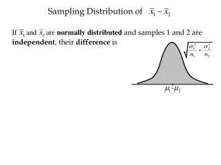
14. SAMPLING FROM THE NORMAL DISTRIBUTION • Let X1, X2,…,Xn be a r.s. of size n from a N(X,X2) distribution and let Y1,Y2,…,Ym be a r.s. of size m from an independent N(Y,Y2). • If we are interested in comparing the variability of the populations, one quantity of interest would be the ratio

15. SAMPLING FROM THE NORMAL DISTRIBUTION • The F distribution allows us to compare these quantities by giving the distribution of • If X~Fp,q, then 1/X~Fq,p. • If X~tq, then X2~F1,q.

16. X Random Variable (Population) Distribution Sample Mean Distribution CENTRAL LIMIT THEOREM If a random sample is drawn from any population, the sampling distribution of the sample mean is approximately normal for a sufficiently large sample size. The larger the sample size, the more closely the sampling distribution of X will resemble a normal distribution. Random Sample (X1, X2, X3, …,Xn)

17. Sampling Distribution of the Sample Mean If X is normal, is normal.If X isnon-normal,is approximately normally distributed for sample size greater than or equal to 30.

18. EXAMPLE 1 • The amount of soda pop in each bottle is normally distributed with a mean of 32.2 ounces and a standard deviation of 0.3 ounces. • Find the probability that a bottle bought by a customer will contain more than 32 ounces. • Solution • The random variable X is the amount of soda in a bottle. 0.7486 m = 32.2 x = 32

19. 0.7486 x = 32 m = 32.2 EXAMPLE 1 (contd.) • Find the probability that a carton of four bottles will have a mean of more than 32 ounces of soda per bottle. • Solution • Define the random variable as the mean amount of soda per bottle. 0.9082

20. ^ p The number of successes X n = Sampling Distribution of a Proportion • The parameter of interest for nominal data is the proportion of times a particular outcome (success) occurs. • To estimate the population proportion ‘p’ we use the sample proportion. The estimate of p =

21. ^ p ^ p Sampling Distribution of a Proportion • Since X is binomial, probabilities about can be calculated from the binomial distribution. • Yet, for inference about we prefer to use normal approximation to the binomial whenever it approximation is appropriate.

22. Approximate Sampling Distribution of a Sample Proportion • From the laws of expected value and variance, it can be shown that E( ) = p and V( )=p(1-p)/n • If both np ≥ 5 and n(1-p) ≥ 5, then • Z is approximately standard normally distributed.

23. EXAMPLE • A state representative received 52% of the votes in the last election. • One year later the representative wanted to study his popularity. • If his popularity has not changed, what is the probability that more than half of a sample of 300 voters would vote for him?

24. EXAMPLE (contd.) Solution • The number of respondents who prefer the representative is binomial with n = 300 and p = .52. Thus, np = 300(.52) = 156 andn(1-p) = 300(1-.52) = 144 (both greater than 5)