Download
1 / 59
590 likes | 702 Vues
Learn how sampling distributions impact statistical analysis, how to calculate margin of error, interpret sample means, and determine sampling error for reliable conclusions. In-depth guide with examples.

E N D
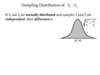
A Sampling Distribution The way our means would be distributed if we collected a sample, recorded the mean and threw it back, and collected another, recorded the mean and threw it back, and did this again and again, ad nauseam!
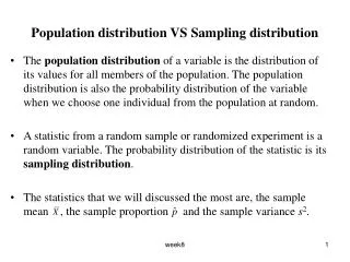
A Sampling Distribution From Vogt: A theoretical frequency distribution of the scores for or values of a statistic, such as a mean. Any statistic that can be computed for a sample has a sampling distribution. A sampling distribution is the distribution of statistics that would be produced in repeated random sampling (with replacement) from the same population. It is all possible values of a statistic and their probabilities of occurring for a sample of a particular size. Sampling distributions are used to calculate the probability that sample statistics could have occurred by chance and thus to decide whether something that is true of a sample statistic is also likely to be true of a population parameter.
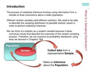
A Sampling Distribution We are moving from descriptive statistics to inferential statistics. Inferential statistics allow the researcher to come to conclusions about a population on the basis of descriptive statistics about a sample.
A Sampling Distribution For example: Your sample says that a candidate gets support from 47%. Inferential statistics allow you to say that the candidate gets support from 47% of the population with a margin of error of +/- 4%. This means that the support in the population is likely somewhere between 43% and 51%.
A Sampling Distribution Margin of error is taken directly from a sampling distribution. It looks like this: 95% of Possible Sample Means 47% 43% 51% Your Sample Mean
A Sampling Distribution Let’s create a sampling distribution of means… Take a sample of size 1,500 from the US. Record the mean income. Our census said the mean is $30K. $30K
A Sampling Distribution Let’s create a sampling distribution of means… Take another sample of size 1,500 from the US. Record the mean income. Our census said the mean is $30K. $30K
A Sampling Distribution Let’s create a sampling distribution of means… Take another sample of size 1,500 from the US. Record the mean income. Our census said the mean is $30K. $30K
A Sampling Distribution Let’s create a sampling distribution of means… Take another sample of size 1,500 from the US. Record the mean income. Our census said the mean is $30K. $30K
A Sampling Distribution Let’s create a sampling distribution of means… Take another sample of size 1,500 from the US. Record the mean income. Our census said the mean is $30K. $30K
A Sampling Distribution Let’s create a sampling distribution of means… Take another sample of size 1,500 from the US. Record the mean income. Our census said the mean is $30K. $30K
A Sampling Distribution Let’s create a sampling distribution of means… Let’s repeat sampling of sizes 1,500 from the US. Record the mean incomes. Our census said the mean is $30K. $30K
A Sampling Distribution Let’s create a sampling distribution of means… Let’s repeat sampling of sizes 1,500 from the US. Record the mean incomes. Our census said the mean is $30K. $30K
A Sampling Distribution Let’s create a sampling distribution of means… Let’s repeat sampling of sizes 1,500 from the US. Record the mean incomes. Our census said the mean is $30K. $30K
A Sampling Distribution Let’s create a sampling distribution of means… Let’s repeat sampling of sizes 1,500 from the US. Record the mean incomes. Our census said the mean is $30K. The sample means would stack up in a normal curve. A normal sampling distribution. $30K
A Sampling Distribution Say that the standard deviation of this distribution is $10K. Think back to the empirical rule. What are the odds you would get a sample mean that is more than $20K off. The sample means would stack up in a normal curve. A normal sampling distribution. $30K -3z -2z -1z 0z 1z 2z 3z
A Sampling Distribution Say that the standard deviation of this distribution is $10K. Think back to the empirical rule. What are the odds you would get a sample mean that is more than $20K off. The sample means would stack up in a normal curve. A normal sampling distribution. 2.5% 2.5% $30K -3z -2z -1z 0z 1z 2z 3z
A Sampling Distribution Social Scientists usually get only one chance to sample. Our graphic display indicates that chances are good that the mean of our one sample will not precisely represent the population’s mean. This is called sampling error. If we can determine the variability (standard deviation) of the sampling distribution, we can make estimates of how far off our sample’s mean will be from the population’s mean.
A Sampling Distribution Knowing the likely variability of the sample means when repeatedly sampling gives us a context within which to judge how much we can trust the number we got from our sample. For example, if the variability is low, , we can trust our number more than if the variability is high, .
A Sampling Distribution Which sampling distribution has the lower variability or standard deviation? a b Now a definition! The standard deviation of a normal sampling distribution is called the standard error. The first sampling distribution above, a, has a lower standard error.
A Sampling Distribution Statisticians have found that the standard error of a sampling distribution is quite directly affected by the number of cases in the sample(s), and the variability of the population distribution. Population Variability: For example, Americans’ incomes are quite widely distributed, from $0 to Bill Gates’. Americans’ car values are less widely distributed, from about $50 to about $50K. The standard error of the latter’s sampling distribution will be a lot less variable.
A Sampling Distribution The sample size affects the sampling distribution: Standard error = population standard deviation / square root of sample size Y-bar= /n
A Sampling Distribution Standard error = population standard deviation / square root of sample size Y-bar= /n IF the population income were distributed with mean, = $30K with standard deviation, = $10K …the sampling distribution changes for varying sample sizes n = 2,500, Y-bar= $10K/50 = $200 n = 25, Y-bar= $10K/5 = $2,000 $30k
A Sampling Distribution Some rules about the sampling distribution of the mean… • For a random sample of size n from a population having mean and standard deviation , the sampling distribution of Y-bar (glitter-bar?) has mean and standard error Y-bar = /n • The Central Limit Theorem says that for random sampling, as the sample size n grows, the sampling distribution of Y-bar approaches a normal distribution. • The sampling distribution will be normal no matter what the population distribution’s shape as long as n > 30. • If n < 30, the sampling distribution is likely normal only if the underlying population’s distribution is normal. • As n increases, the standard error (remember that this word means standard deviation of the sampling distribution) gets smaller. • Precision provided by any given sample increases as sample size n increases.
A Sampling Distribution So we know in advance of ever collecting a sample, that if sample size is sufficiently large: • Repeated samples would pile up in a normal distribution • The sample means will center on the true population mean • The standard error will be a function of the population variability and sample size • The larger the sample size, the more precise, or efficient, a particular sample is • 95% of all sample means will fall between +/- 2 s.e. from the population mean
A Sampling Distribution So why are sampling distributions less variable when sample size is larger? Example 1: • Think about what kind of variability you would get if you collected income through repeated samples of size 1 each. • Contrast that with the variability you would get if you collected income through repeated samples of size N – 1 (or 300 million minus one) each.
A Sampling Distribution So why are sampling distributions less variable when sample size is larger? Example 1: • Think about what kind of variability you would get if you collected income through repeated samples of size 1 each. • Contrast that with the variability you would get if you collected income through repeated samples of size N – 1 (or 300 million minus one) each. Example 2: • Think about drawing the population distribution and playing “darts” where the mean is the bull’s-eye. Record each one of your attempts. • Contrast that with playing “darts” but doing it in rounds of 30 and recording the average of each round. • What kind of variability will you see in the first versus the second way of recording your scores. …Now, do you trust larger samples to be more accurate?
A Sampling Distribution An Example: A population’s car values are = $12K with = $4K. Which sampling distribution is for sample size 625 and which is for 2500? What are their s.e.’s? 95% of M’s 95% of M’s ? $12K ? ? $12K ? -3 -2 -1 0 1 2 3 -3-2-1 0 1 2 3
A Sampling Distribution An Example: A population’s car values are = $12K with = $4K. Which sampling distribution is for sample size 625 and which is for 2500? What are their s.e.’s? s.e. = $4K/25 = $160 s.e. = $4K/50 = $80 (625 = 25) (2500 = 50) 95% of M’s 95% of M’s $11,840 $12K $12,320 $11,920$12K $12,160 -3 -2 -1 0 1 2 3 -3-2-1 0 1 2 3
A Sampling Distribution A population’s car values are = $12K with = $4K. Which sampling distribution is for sample size 625 and which is for 2500? Which sample will be more precise? If you get a particularly bad sample, which sample size will help you be sure that you are closer to the true mean? 95% of M’s 95% of M’s $11,840 $12K $12,320 $11,920$12K $12,160 -3 -2 -1 0 1 2 3 -3-2-1 0 1 2 3
Estimation Before we collect our sample, we know: Repeated sampling sample means would stack up in a normal curve, Centered on the true population mean, With a standard error (measure of dispersion) that depends on 1. population standard deviation 2. sample size -3z -2z -1z 0z 1z 2z 3z
Estimation But we do not know: 1. True Population Mean 2. Population Standard Deviation Repeated sampling sample means would stack up in a normal curve, Centered on the true population mean, With a standard error (measure of dispersion) that depends on 1. population standard deviation 2. sample size -3z -2z -1z 0z 1z 2z 3z
Estimation Will our sample be one of these (accurate)? Or one of these (inaccurate)? -3z -2z -1z 0z 1z 2z 3z
Estimation Which is more likely? accurate? or inaccurate? -3z -2z -1z 0z 1z 2z 3z 68% 95%
Estimation We’re most likely to get close to the true population mean… Our sample’s mean is the best guess of the population mean, but it is not precise. -3z -2z -1z 0z 1z 2z 3z 68% 95%
Estimation And if we increase our sample size (n)… -3z -2z -1z 0z 1z 2z 3z 68% 95%
Estimation And if we increase our sample size our sample mean is an even better estimate of the population mean, we are more precise! -3 -2 -1 0 1 2 3 -3z -2z -1z 0z 1z 2z 3z 68% 95%
Estimation We know that the standard deviation of this pile of samples (standard error) equals the population standard deviation () divided by the square root of the sample size (n). -3 -2 -1 0 1 2 3 68% 95%
Estimation But we do not know the population standard deviation! What is our best guess of that? -3 -2 -1 0 1 2 3 68% 95%
Estimation Our best guess of the population standard deviation is our sample’s s.d.! On average, this s.d. gives population . In fact, when we calculate that, we use “n – 1” to make our “estimate” larger to reflect that dispersion of a sample is smaller than a population’s. (Yi – Y)2 s.d. = n - 1 = Cases in the sample 0 5 10 15 20 25 30 35 0 5 10 15 20 25 30 35 Population Dispersion Sample Dispersion
Estimation So now we know that we can use the sample standard deviation to stand in for the population’s standard deviation. So we can use run the formula for standard error with that s.d. estimate and get a good estimate s.e = of the dispersion of the n sampling distribution. -3 -2 -1 0 1 2 3 68% 95%
Estimation Now we know how far off our sample mean is likely to be from the true population mean! 68% of means will be within +/- 1 s.e. 95% of means will be within +/- 2 s.e. s.d. s.e. = n -3 -2 -1 0 1 2 3 68% 95%
Estimation For example, if we took GPAs from a sample of 625 students and our s.d. was .50… 68% of means will be within +/- 1(.02) 95% of means will be within +/- 2 (.02) .5 s.e. = 625 = 0.02 -3 -2 -1 0 1 2 3 68% 95%
Estimation For example, if we took GPAs from a sample of 625 students and our s.d. was .50… If our sample were this one( ), our estimate of the mean would be right! .5 s.e. = 625 = 0.02 -3 -2 -1 0 1 2 3 68% 95%
Estimation For example, if we took GPAs from a sample of 625 students and our s.d. was .50… But what if it were this one( )? We’d be slightly wrong, but well within +/- 2 (.02) 95% of samples would be! .5 s.e. = 625 = 0.02 -3 -2 -1 0 1 2 3 68% 95%
Estimation A sample’s mean is the best estimate of the population mean. But what if we base our estimate on this erroneous sample? But what if it were this one( )? We’d be slightly wrong, but well within +/- 2 s.d. 95% of samples would be! s.d. s.e. = n -3 -2 -1 0 1 2 3 68% 95%
Estimation Well, let’s center our sampling distribution on our sample’s mean( ). Check it Out! The true mean falls within the 95% bracket. s.d. s.e. = n -3 -2 -1 0 1 2 3 68% 95%
Estimation What if the sample we collected were this one ( )? Check it Out! The true mean falls within the 95% bracket. s.d. s.e. = n -3 -2 -1 0 1 2 3 68% 95%
Estimation The sampling distribution allows us to: 1. Be humble and admit that our sample statistic may not be the population’s and 2. Forms a measuring device with which we can determine a range where the true population mean is likely to fall... this is called a confidence interval.
Estimation If you calculate your sampling distribution’s standard error, you can form a device that tells you that if your sample mean is wrong, there is a documented a range in which the true population mean is likely 2Xist. Check it Out! The true mean falls within the 95% bracket. s.d. s.e. = n -3 -2 -1 0 1 2 3 68% 95%