Sampling Distribution of a Sample Mean

1. Sampling Distribution of a Sample Mean Lecture 28 Section 8.4 Fri, Oct 20, 2006

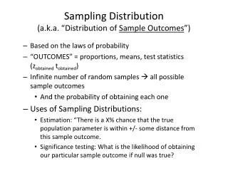
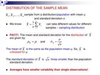
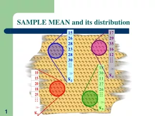
2. Sampling Distribution of the Sample Mean • Sampling Distribution of the Sample Mean– The distribution of sample means over all possible samples of the size n from the population.

3. With or Without Replacement? • If the sample size is small in relation to the population size (< 5%), then it does not matter whether we sample with or without replacement. • The calculations are simpler if we sample with replacement. • In any case, we are not going to worry about it.

4. Example • Suppose a population consists of the numbers {6, 12, 18}. • Using samples of size n = 1, 2, or 3, find the sampling distribution ofx. • Draw a tree diagram showing all possibilities.

5. The Tree Diagram (n = 1) • n = 1 mean = 6 6 mean = 12 12 mean = 18 18

6. The Sampling Distribution (n = 1) • The sampling distribution ofx is • The parameters are •  = 12 • 2 = 24

7. The Sampling Distribution (n = 3) • The shape of the distribution: density 1/3 mean 6 8 10 12 14 16 18

8. The Tree Diagram (n = 2) mean 6 6 12 6 9 12 18 6 9 12 12 12 15 18 6 12 18 12 15 18 8

9. The Sampling Distribution (n = 2) • The sampling distribution ofx is • The parameters are •  = 12 • 2 = 12

10. The Sampling Distribution (n = 3) • The shape of the distribution: density 3/9 2/9 1/9 mean 6 8 10 12 14 16 18

11. The Tree Diagram (n = 3) mean 6 6 6 12 8 18 10 6 8 12 6 12 10 18 12 6 10 12 12 18 14 18 6 8 6 12 10 18 12 6 10 12 12 12 12 18 14 6 12 18 12 14 18 16 6 10 6 12 12 18 14 18 6 12 12 12 14 18 16 6 14 12 18 16 18 18

12. The Sampling Distribution (n = 3) • The sampling distribution ofx is • The parameters are •  = 2 • 2 = 8

13. The Sampling Distribution (n = 3) • The shape of the distribution: density 9/27 6/27 3/27 mean 6 8 10 12 14 16 18

14. Sampling Distributions • Run the program Central Limit Theorem for Means.exe. • Use n = 30 and population = {6, 12, 18} • Generate 100 samples.

15. 100 Samples of Size n = 30  = 0.75  = 0.079

16. Observations and Conclusions • Observation #1: The values ofx are clustered around . • Conclusion #1:x is probably close to .

17. Larger Sample Size • Now we will select 100 samples of size 120 instead of size 30. • Run the program Central Limit Theorem for Means.exe. • Pay attention to the spread (standard deviation) of the distribution.

18. 100 Samples of Size n = 120  = 0.75  = 0.0395

19. Observations and Conclusions • Observation #2: As the sample size increases, the clustering is tighter. • Conclusion #2-1: Larger samples give more reliable estimates. • Conclusion #2-2: For sample sizes that are large enough, we can make very good estimates of the value of .

20. Larger Sample Size • Now we will select 10000 samples of size 120 instead of only 100 samples. • Run the program Central Limit Theorem for Means.exe. • Pay attention to the shape of the distribution.

21. 10,000 Samples of Size n = 120  = 0.75  = 0.0395

22. 10,000 Samples of Size n = 120

23. More Observations and Conclusions • Observation #3: The distribution ofx appears to be approximately normal. • Conclusion #3: We can use the normal distribution to calculate just how close to  we can expectx to be.

24. One More Conclusion • However, we must know the values of  and  for the distribution ofx. • That is, we have to quantify the sampling distribution ofx.

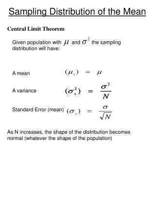
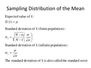
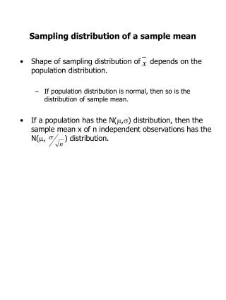
25. The Central Limit Theorem • Begin with a population that has mean  and standard deviation . • For sample size n, the sampling distribution of the sample mean is approximately normal with

26. The Central Limit Theorem • The approximation gets better and better as the sample size gets larger and larger. • That is, the sampling distribution “morphs” from the distribution of the original population to the normal distribution. • For many populations, the distribution is almost exactly normal when n  10. • For almost all populations, if n 30, then the distribution is almost exactly normal.

27. The Central Limit Theorem • Therefore, if the original population is exactly normal, then the sampling distribution of the sample mean is exactly normal for any sample size. • This is all summarized on pages 536 – 537.

28. Example

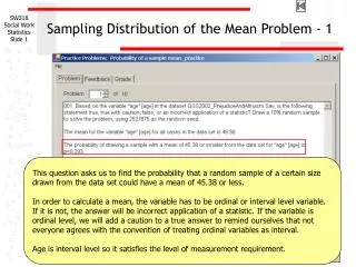
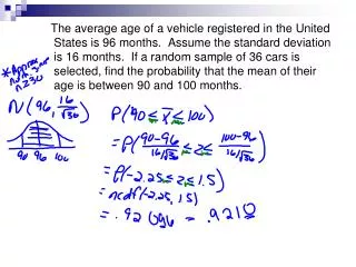
29. Example • Over the course of the semester, I sample (grade) approximately 100 homework problems per student. • Thus, n = 100. • What is the sampling distribution of the homework average (for the typical student)?

30. Example • Based on the Central Limit Theorem for Means, the sampling distribution • Is normally distributed (n  30) • Has a mean of 7.3 points. • Has a standard deviation of 2.9/100 = 0.29 points. • On a 100-point scale, that would be • An average of 73. • A standard deviation 2.9.

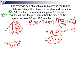
31. Example • What is the probability that a student’s homework average (100 sampled problems) will be within 5 points of his true average for all problems?

32. Example • For the typical student, that would be a homework average between 68 and 78. • normalcdf(68, 78, 73, 2.9) = 0.9153, or about 92%

33. Point of Fact • Since the sample size (n = 100) is a sizable fraction of the population size (N = 400) and we are sampling without replacement, we should take into account the “finite population correction factor” of (N – n)/(N – 1) for the variance ofx.

34. Point of Fact • For n = 100 and N = 400, this factor is 0.8671. • Thus, in fact, the typical standard deviation is only about 0.251, or 2.51 points out of 100. • Recompute: normalcdf(68, 78, 73, 2.51) = 0.9536, or 95.36%.