Download
1 / 8
80 likes | 177 Vues
Delve into the properties of sampling distribution and understand how sample means are calculated and analyzed for probability statements. Learn about normal distribution, mean, standard error, Z-values, and making probability statements in statistical analysis.

E N D
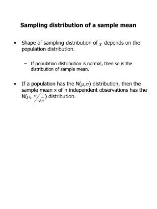
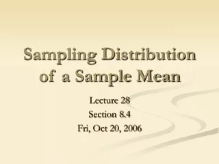
The Sampling Distribution of the Sample Mean AGAIN – with a new angle
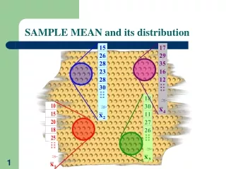
Say I have a population of 20 students in a class and their ages are: 6 are 18, 6 are 19, 6 are 20, 1 is 24 and 1 is 30. Then some population parameters are: Now, in the real world when we have a population and we know some parameters like the mean and standard deviation, then the information can be used to make probability statements about the likelihood of certain events. But, here I want to develop some ideas, so I want you to consider taking a sample of size 9 from the population of 20. You can see if in a sample of 9 I had the 6 18 year olds and 3 19 year olds the sample mean would be 18.33 The sample mean would be different if we had a different 9 people make the sample. So the sample mean depends on the sample chosen. If we had 6 19 year olds and 3 20 year olds the mean would be 19.33
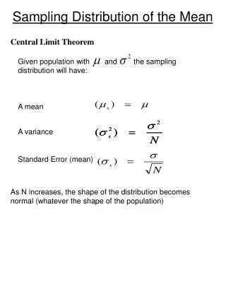
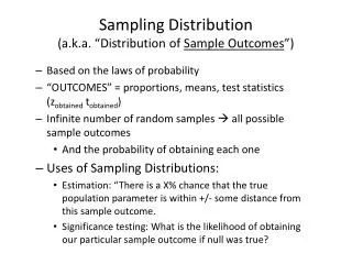
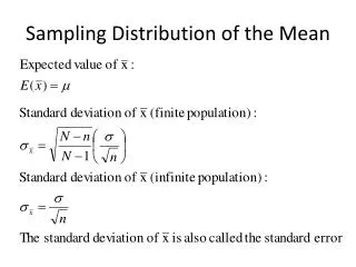
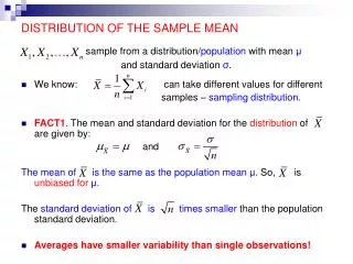
Again, remember that we usually would not take more than 1 sample of size 9 because it would be time consuming and costly. But in theory we can imagine taking all the different samples of size 9 from the 20 people and for each sample we could calculate the mean. We could then think about the distribution of sample means – what is called a sampling distribution. The theoretical distribution of sample means has three properties: 1) It is a normal distribution, 2) Has the same mean as the mean in the population, 3) Has standard error, which is just the name of the standard deviation of a sampling distribution, equal to the standard deviation in the population divided by the square root of the sample size. In the example I cooked up the distribution of sample means is normal, has mean = 19.8, and has standard error = 2.69/sqrt(9) = .9
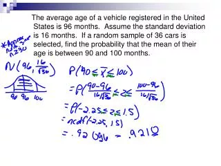
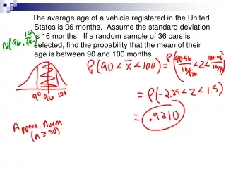
So, what have we accomplished? Well, we know the sample mean would likely be different for different samples from the population and therefore the sample mean really has a distribution. Once we know something is normally distributed than we can make probability statements about that something. Here we could make statements about how likely we are to get a sample mean in a certain neighborhood of the number line. What is the probability of getting a sample mean between 19 and 20? The value 19 has Z=(19 – 19.8)/(2.69/sqrt(9)) = -.83, and the value 20 has Z = (20 – 19.8)/(2.69/sqrt(9)) = .21. Prob(19<mean<20) = .5832 – (1-7967) = .3799.
So, in theory sample means have a distribution and once we know the properties of the distribution we can make probability statements about the likelihood of getting a mean in a certain interval. NOTE: when you work with a variable in the population the z value uses the standard deviation in the population… But when you are working with sample means and you calculate a z you use the standard deviation in the population divided by the square root of the sample size. Making probability statements about either the variable itself or about the sample means follows the same procedure except you have to use the appropriate value in the z calculation.
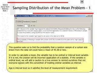
Problem 7.2 page 216 X bar has a normal distribution with mean = 50 and standard error = 5/10 = .5 a. 47 has Z = (47 – 50)/.5 = -6.00 and from the table we see P(X bar < 47) = .000000001 b. 49.5 has Z = (49.5 – 50)/.5 = -1.00 and in the table we have the area to the left of .1587. So, .1587 minus .000000001 = .1587 for our purposes. c. 51.1 has Z = (51.1 – 50)/.5 = 2.20 and in the table we see the value .9861. Since this is the area below 51.1 we take 1 minus this to get the area above of .0139
Problem 7.2 page 277 d. We are looking for the X bar that has .3500 to the right of it, or .6500 to the left of it. The Z with .6500 to the left is .39 (closest) and thus X bar is found from .39 = (X bar – 50)/.5, or X bar = 50 + .5(.39) = 50.195
Problem 8 page 216 The standard error of the mean is .4/sqrt(16) = .4/4 = .1 a. The Z for 3 is (3 – 3.1)/.1 = -.1/.1 = -1.00. The area to the left of this is .1587. But at least 3 means 3 or more so we need 1 minus .1587 = .8413 b. We need to find the Z that has an area = .8500. The closest Z is 1.04 and then to find the value we take 1.04=(value – 3.1)/.1 or value = .1(1.04) + 3.1 = .3204. c. The population is approximately normal. d. With 64 as the sample size the standard error is .4/8 = .05 and to get the value we take 1.04 = (value – 3.1)/.05, or value = .05(1.04) + 3.1 = 3.152.