Sampling Distribution of the Mean Problem - 1
290 likes | 567 Vues
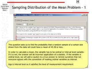
Sampling Distribution of the Mean Problem - 1. This question asks us to find the probability that a random sample of a certain size drawn from the data set could have a mean of 45.38 or less.

Sampling Distribution of the Mean Problem - 1
E N D
Presentation Transcript
Sampling Distribution of the Mean Problem - 1 This question asks us to find the probability that a random sample of a certain size drawn from the data set could have a mean of 45.38 or less. In order to calculate a mean, the variable has to be ordinal or interval level variable. If it is not, the answer will be incorrect application of a statistic. If the variable is ordinal level, we will add a caution to a true answer to remind ourselves that not everyone agrees with the convention of treating ordinal variables as interval. Age is interval level so it satisfies the level of measurement requirement.
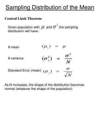
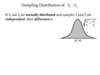
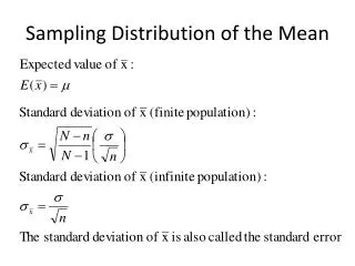
Sampling Distribution of the Mean Problem - 2 The probability that a random sample has a specific mean is based on its location within the sampling distribution of the means of all the possible samples we could draw from the data set (just like a zscore for one case in a sample). The mean of the sampling distribution is the population mean, or the mean of all cases in the data set. Our problems compare the mean of one sample SPSS will draw (45.38) to the population mean (46.58).
Sampling Distribution of the Mean Problem - 3 Since the distribution of sampling means is based on the normal distribution, the correct probability for any specific mean value assumes that the variable follows a normal distribution. To verify that our data satisfies this assumption, we will also compute the skewness and kurtosis of the distribution of all cases in the data set.
Computing mean, skewness, and kurtosis To compute the mean, skewness, and kurtosis, select Descriptive Statistics > Descriptives in SPSS.
Descriptive statistics: selecting variable First, move the variable age to the Variables list box. Second, click on the Options button to select the statistics.
Descriptive statistics: selecting statistics First, mark the check boxes for Mean, Kurtosis, and Skewness. Second, click on the Continue button to close the options window.
Complete the request for the statistics To complete the request for the statistics, click on the OK button.
The population mean Since we are treating all of the cases in the data set as the population in these problems, the population mean is 46.58. The population mean stated in the problem is 46.58, so our problem is true so far. We will need the numeric value for the population mean when we compute the probability of the sample mean.
Testing for normality Obtaining accurate probabilities for the sampling distribution of means assumes that the variable is normally distributed. The "age" [age] satisfied the criteria for a normal distribution. The skewness of the distribution (.454) was between -1.0 and +1.0 and the kurtosis of the distribution (-.720) was between -1.0 and +1.0. If we did not satisfy the requirements for a normal distribution, we might still be able to compute a correct probability, using the Central Limit Theorem. In this problem, we don’t need the Central Limit Theorem, but if we did, we would need to draw the sample and compute the sample mean.
Drawing a sample: setting the seed or starting random number Setting the random number seed tells SPSS what number to start with when it draws a random subset of cases. If you do not use the same seed that I did, you will not get the same sample of cases, and your answers will probably not match the problems. To set a random number seed, go to Transform > Random Number Seed… in SPSS.
Drawing a sample: entering the random seed number To create a random process using a specific number, 2527675 in this problem, as a random number seed, click on “Set seed to:” and type in the number you want. When you click on OK, the seed will be set, but you will get no feedback from SPSS telling you that this has been done.
Drawing a random sample:selecting the cases to include Now, we have to tell SPSS to select 10% of the whole data set as the sample. Select the command: Data > Select Cases…
Drawing a random sample:specifying a random selection of cases First, click on the option button Random sample of cases. Second, click on the Sample button to specify the size of the sample.
Drawing a random sample:specifying the size of the random sample The problem calls for us to draw a 10% random sample. Type 10 in the text box in front of the % symbol to specify the size of the sample. Then, click on the Continue button to close the dialog box.
Drawing a random sample:completing the specifications SPSS repeats our request next to the Sample button. Click on the OK button to complete the sampling specifications and draw the sample.
Cases included in the sample SPSS indicates which cases are excluded from the sample by drawing a diagonal line through the case number, as shown for case 1, 2, 3, etc. The cases which are included in the random sample drawn by SPSS do not have a line across the case number. CaseID 40 on row 11 is included in the sample.
The probability of a sample mean Having drawn a 10% sample of the cases in the data set, we can calculate the statistics for the sample. The SPSS procedure “One-Sample T Test” computes the probability of a sample mean from a population. Select: Compare Means > One-Sample T Test from the SPSS menus
Specifications for One-Sample T Test First, move the variable “age” to the list box for Test Variable(s). Third, click on the OK button to complete the request. Second, type the population mean that we found in the statistics for all cases in the data set in the text box for the Test Value. This is the population mean we found back on slide 8.
Output for One-Sample T Test The mean for the random sample selected by SPSS was 45.38. This corresponds to the sample mean the problem asks us about. The number of cases in the 10% random sample selected by SPSS was 61. If we did not satisfy the skewness and kurtosis criteria for normality, we would compare the sample size to the Central Limit Theorem minimum sample size to see if we can satisfy the normality assumption with the Central Limit Theorem (sample has 50 or more cases).
The probability of the sample mean The probability associated with a sample mean of 45.38 from a population with a mean of 46.58 is given by the Sig. (2-tailed) cell in the one-sample test table. This probability, or p-value, is the probability that the sample mean is larger or smaller than the population mean. In our problems we are interested in only one direction, smaller or larger as specified by the problem, so we divide this sig value by 2, 0.586 ÷ 2 = 0.293.
Answering the problem The answer to the problem is true. The probability the a 10% random sample drawn by SPSS could have a mean of 45.38 or smaller was 0.293. The level of measurement was satisfied because the variable was interval level. The variable satisfied the normality assumption by having a value for skewness and kurtosis between -1.0 and +1.0.
Picturing the Sampling Distribution 15 10 5 0 Population Mean: 46.58 Mean of this sample: 45.38 S.D. = 2.19 Mean of Means= 46.58 Sample size = 61 Frequency 42 43 44 45 46 47 48 49 50 51 We calculated the p-value of this part of the distribution. Sample Means
Restoring all cases to the data set - 1 When we have completed a problem, we need to restore all of the cases to the data set before working the next problem. Select the command: Data > Select Cases…
Restoring all cases to the data set - 2 First, click on the option button All Cases. Second, click on the OK button.
Restoring all cases to the data set - 3 All of the slash marks through the case numbers have been removed. Statistics will now be calculated on all cases in the data set.
Steps in solving sampling distribution of means problems - 1 The following is a guide to the decision process for answering homework problems about sampling distributions of means: Is the variable ordinal or interval level? Incorrect application of a statistic No Yes Compute the mean, skewness, and kurtosis for the population (all cases in the data set).
Steps in solving sampling distribution of means problems - 2 Assumption of normality satisfied? (skew, kurtosis between -1.0 and + 1.0) Yes No Draw the random sample from the data set and compute the sample statistics Draw the random sample from the data set and compute the sample statistics Sample size 50+ so Central Limit Theorem applies? Incorrect application of a statistic No Yes
Steps in solving sampling distribution of means problems - 3 Divide the 2-tailed Sig. value in half to find the one direction probability. Statistical values for population mean, sample mean, and p-value correct? No False Yes No Is the variable ordinal level? True Yes True with caution