Download
1 / 38
440 likes | 948 Vues
Chapter 6 Sampling Distributions( 样本分布 ). The Sampling Distribution of the Sample Mean The Sampling Distribution of the Sample Proportion. Sample Mean. Example: The law firm of Hoya and Associates has five partners. At their weekly partners meeting each reported the number of

E N D
Chapter 6 Sampling Distributions(样本分布) • The Sampling Distribution of the Sample Mean • The Sampling Distribution of the Sample Proportion
Sample Mean Example: The law firm of Hoya and Associates has five partners. At their weekly partners meeting each reported the number of hours they billed clients for their services last week. If two partners are selected randomly, how many different samples are possible? A total of 10 different samples Chapter 6 Sampling Distributions
As a sampling distribution Different samples of the same size from the same population will yield different sample means
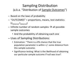
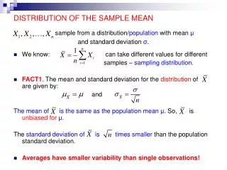
Sample Mean • Let there be a population of units of size N • Consider all its samples of a fixed size n (n<N) • For all possible samples of size n, we obtain a population of sample means. That is, is a random variable which may have all these means as its values • Before we draw the sample, the sample mean is a random variable. • We consider the probability distribution of the random variable , i.e., the probability distribution for the population of sample means Chapter 6 Sampling Distributions
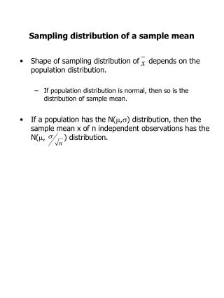
Section 6.1 The Sampling Distribution of the Sample Mean The sampling distribution of the samplemean is the probability distribution of the population of the sample means obtainable from all possible samples of size n from a population of size N. Chapter 6 Sampling Distributions
Example 6.1 The Stock Return Case • We have a population of the percent returns from six stocks • In order, the values of % return are: 10%, 20%, 30%, 40%, 50%, and 60% • Label each stock A, B, C, …, F in order of increasing % return • The mean rate of return is 35% with a standard deviation of 17.078% • Any one stock of these stocks is as likely to be picked as any other of the six • Uniform distribution with N = 6 • Each stock has a probability of being picked of 1/6 Chapter 6 Sampling Distributions
The Stock Return Case ﹟2 Chapter 6 Sampling Distributions
The Stock Return Case ﹟3 • Now, select all possible samples of size n = 2 from this population of stocks of size N = 6 • That is, select all possible pairs of stocks • How to select? • Sample randomly • Sample without replacement • Sample without regard to order Chapter 6 Sampling Distributions
The Stock Return Case ﹟4 • Result: There are 15 possible samples of size n = 2 • Calculate the sample mean of each and every sample • For example, if we choose the two stocks with returns 10% and 20%, then the sample mean is 15% Chapter 6 Sampling Distributions
The Stock Return Case ﹟5 Chapter 6 Sampling Distributions
Observations • The population of N = 6 stock returns has a uniform distribution. • But the histogram of n = 15 sample mean returns: • Seems to be centered over the same mean return of 35%, and • Appears to be bell-shaped and less spread out than the histogram of individual returns Chapter 6 Sampling Distributions
Example 6.2 Sampling all the stocks • Consider the population of returns of all 1,815 stocks listed on NYSE for 1987 • See Figure 6.2(a) on next slide • The mean rate of return was –3.5% with a standard deviation of 26% • Draw all possible random samples of size n= 5 and calculate the sample mean return of each • Sample with a computer • See Figure 6.2(b) on next slide Chapter 6 Sampling Distributions
Observations • Both histograms appear to be bell-shaped and centered over the same mean of –3.5% • The histogram of the sample mean returns looks less spread out than that of the individual returns • Statistics • Mean of all sample means:m=m= -3.5% • Standard deviation of all possible means: Chapter 6 Sampling Distributions
General Conclusions • If the population of individual items is normal, then the population of all sample means is also normal • Even if the population of individual items is not normal, there are circumstances that the population of all sample means is normal (see Central Limit Theorem(中心极限定理)later) Chapter 6 Sampling Distributions
General Conclusions • The mean of all possible sample means equals the population mean • That is,m=m • The standard deviation sx of all sample means is less than the standard deviation of the population • That is,s<s • Each sample mean averages out the high and the low measurements, and so are closer to m than many of the individual population measurements Chapter 6 Sampling Distributions
The empirical rule holdsfor the sampling distribution of the sample mean • 68.26% of all possible sample means are within (plus or minus) one standard deviationsofm • 95.44% of all possible observed values of x are within (plus or minus) twosofm • In the example., 95.44% of all possible sample mean returns are in the interval [-3.5 ± (211.63)]= [-3.5 ± 23.26] • That is, 95.44% of all possible sample means are between -26.76% and 19.76% • 99.73% of all possible observed values of x are within (plus or minus) threesofm Chapter 6 Sampling Distributions
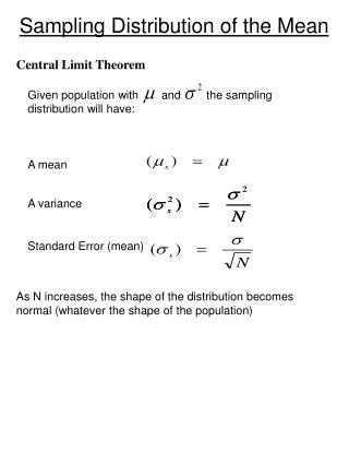
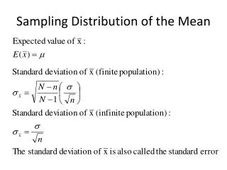
Properties of the SamplingDistribution of the Sample Mean #1 • If the population being sampled is normal, then so is the sampling distribution of the sample mean, • The mean of the sampling distribution of is • m = m • That is, the mean of all possible sample means is the same as the population mean Chapter 6 Sampling Distributions
Properties of the SamplingDistribution of the Sample Mean #2 • The variance s2 of the sampling distribution of is • That is, the variance of the sampling distribution of is • directly proportional to the variance of the population, and • inversely proportional to the sample size Chapter 6 Sampling Distributions
Properties of the SamplingDistribution of the Sample Mean #3 • The standard deviation s of the sampling distribution of is • That is, the standard deviation of the sampling distribution of is • directly proportional to the standard deviation of the population, and • inversely proportional to the square root of the sample size Chapter 6 Sampling Distributions
Notes • is the point estimate ofm, and the larger the sample size n, the more accurate the estimate, because when n increases,sdecreases,is more clustered to the population • In order to reduces, take bigger samples! Chapter 6 Sampling Distributions
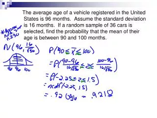
Car Mileage Case Example 6.3 • Population of all midsize cars of a particular make and model • Population is normal with meanmand standard deviations • Draw all possible samples of size n • Then the sampling distribution of the sample mean is normal with meanm=mand standard deviation • In particular, draw samples of size: • n = 5 • n = 49 Chapter 6 Sampling Distributions
So, all possible sample means for n=49 will be more closely clustered around m than the case of n =5 Chapter 6 Sampling Distributions
Central Limit Theorem(中心极限定理)#1 • If the population is non-normal, what is the shape of the sampling distribution of the sample means? • In fact the sampling distribution is approximately normal if the sample is large enough, even if the population is non-normal • by the “Central Limit Theorem” Chapter 6 Sampling Distributions
No matter what is the probability distribution that describes the population, if the sample size n is large enough,then the population of all possible sample means is approximately normal with mean and standard deviation • Further, the larger the sample size n, the closer the sampling distribution of the sample means is to being normal • In other words, the larger n, the better the approximation Chapter 6 Sampling Distributions
X as n large Population Distribution (m, s) (right-skewed) Sampling Distribution of Sample Means (nearly normal) Random Sample (x1, x2, …, xn) Chapter 6 Sampling Distributions
Effect of the Sample Size Example 6.4 The larger the sample size, the more nearly normally distributed is the population of all possible sample means Also, as the sample size increases, the spread of the sampling distribution decreases Chapter 6 Sampling Distributions
How Large? • How large is “large enough?” • If the sample size n is at least 30, then for most sampled populations, the sampling distribution of sample means is approximately normal Refer to Figure 6.6 on next slide • Shown in Fig 6.6(a) is an exponential (right skewed) distribution • In Figure 6.6(b), 1,000 samples of size n = 5 • Slightly skewed to right • In Figure 6.6(c), 1,000 samples with n = 30 • Approximately bell-shaped and normal • If the population is normal, the sampling distribution of is normal regardless of the sample size Chapter 6 Sampling Distributions
Example: Central Limit Theorem Simulation Chapter 6 Sampling Distributions
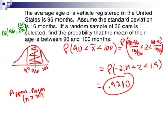
Reasoning from Sample Distribution • Recall from Chapter 2 mileage example,= 31.5531 mpg for a sample of size n=49 • With s = 0.7992 • Does this give statistical evidence that the population meanmis greater than 31 mpg? • That is, does the sample mean give evidence thatmis at least 31 mpg? • Calculate the probability of observing a sample mean that is greater than or equal to 31.5531 mpg ifm= 31 mpg • WantP(> 31.5531 ifm = 31) Chapter 6 Sampling Distributions
Use s as the point estimate for s so that • Then • But z = 4.84 is off the standard normal table • The largest z value in the table is 3.09, which has a right hand tail area of 0.001 Chapter 6 Sampling Distributions
Probability that> 31.5531 when = 31 Chapter 6 Sampling Distributions
z = 4.84 > 3.09, so P(z ≥ 4.84) < 0.001 • That is, ifm= 31 mpg, then fewer than 1 in 1,000 of all possiblesamples have a mean at least as large as observed • Have either of the following explanations: • Ifmis actually 31 mpg, then picking this sample is an almost unbelievable thing OR • mis not 31 mpg • Difficult to believe such a small chance would occur, so conclude that there is strongevidence thatmdoes not equal 31 mpg. • mis in fact larger than 31 mpg Chapter 6 Sampling Distributions
Section 6.2 The Sampling Distribution of the Sample Proportion(样本比例) For a population of units, we select samples of size n, and calculate its proportion for the units of the sample to be fall into a particular category. is a random variable and has its probability distribution. The probability distribution of all possible sample proportions is called the sampling distribution of the sample proportion Chapter 6 Sampling Distributions
the sampling distribution of is • approximately normal, if n is large (meet the conditions that np≥5 and n(1-p)≥5) • has mean • has standard deviation where p is the population proportion for the category Chapter 6 Sampling Distributions
Example 6.5 The Cheese Spread Case • A food processing company developed a new cheese spread spout which may save production cost. If only less than 10% of current purchasers do not accept the design, the company would adopt and use the new spout. • 1000 current purchasers are randomly selected and inquired, and 63 of them say they would stop buying the cheese spread if the new spout were used. So, the sample proportion =0.063. • To evaluate the strength of this evidence, we ask: if p=0.1, what is the probability of observing a sample of size 1000 with sample proportion ≦0.063? Chapter 6 Sampling Distributions
If p=0.10, since n=1000, np≥5 and n(1-p)≥5, is approximately normal with Chapter 6 Sampling Distributions
So, if p=0.1, the chance of observing at most 63 out of 1000 randomly selected customers do not accept the new design is less than 0.001 • But such observation does occur. This means that we have extremely strong evidence that p≠0.1, and p is in fact less than 0.1 • Therefore, the company can adopt the new design Chapter 6 Sampling Distributions