Download
1 / 24
260 likes | 302 Vues
Learn about the properties of point estimators including unbiasedness, consistency, and efficiency. Explore how to compute point estimates and interval estimates in statistical analysis.

E N D
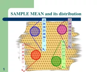
SAMPLE MEAN and its distribution CENTRAL LIMIT THEOREM: If sufficiently large sample is taken from population with any distribution with mean and standard deviation , then sample mean has sample normal distribution N(,2/n) It means that: • sample mean is a good estimate of population mean • with increasing sample size n, standard error SE is lower and estimate of population mean is more reliable
SAMPLE MEAN and its distribution http://onlinestatbook.com/stat_sim/sampling_dist/index.html
ESTIMATORS • point • interval
Properties of Point Estimators • UNBIASEDNESS • CONSISTENCY • EFFICIENCY
Properties of Point Estimators • UNBIASEDNESS • An estimator isunbiased if, based on repeated sampling from the population, the average value of the estimator equals the population parameter. In other words, for an unbiased estimator, the expected value of the point estimator equals the population parameter.
Properties of Point Estimators UNBIASEDNESS
Properties of Point Estimators true value of population parameter individual sample estimates
ZÁKLADNÍ VLASTNOSTI BODOVÝCH ODHADŮ bias of estimates true value of population parameter y – sample estimates M - „average“ of sample estimates
Properties of Point Estimators CONSISTENCY An estimator is consistent if it approaches the unknown population parameter being estimated as the sample size grows larger Consistency implies that we will get the inference right if we take a large enough sample. For instance, the sample mean collapses to the population mean (X̅ → μ) as the sample size approaches infinity (n → ∞). An unbiased estimator is consistent if its standard deviation, or its standard error, collapses to zero as the sample size increases.
Properties of Point Estimators CONSISTENCY
Properties of Point Estimators EFFICIENCY An unbiased estimator is efficient if its standard error is lower than that of other unbiased estimators
Properties of Point Estimators unbiased estimator with small variability (efficient) unbiased estimator with large variability (unefficient)
POINT ESTIMATES Point estimate of population mean: Point estimate of population variance: bias correction
population this distance isunknown (we do not knowtheexactvalueofm) , sowecan not quatifyreliabilityofourestimate sample POINT ESTIMATES
point estimate of unknown population mean computed from sample data– we do not know anything about his distance from real population mean T2 T1 interval estimate of unknown population mean - we suppose, that with probability P =1- population mean is anywhere in this interval of number line INTERVAL ESTIMATES Confidence interval for parametr with confidence level(0,1) is limited by statistics T1 a T2:.
these intervals include real value of population mean (they are „correct“), there will be at least (1- ).100 % these „correct“ estimates this interval does not include real value of population mean (it is „incorrect“), there will be at most (100) % of these „incorrect“ estimates CONFIDENCE LEVEL IN INTERVAL ESTIMATES
1= /2 P = 1 - = 1 – (1 + 2) 2= /2 T1 T2 T TWO-SIDED INTERVAL ESTIMATES 1 a 2 represent statistical risk, that real population parameter is outside of interval (outside the limits T1 a T2
ONE-SIDED INTERVAL ESTIMATES LEFT-SIDED ESTIMATE RIGHT-SIDED ESTIMATE
/2 T one-sided interval estimate P = 1 - T1 /2 T1 T2 two-sided interval estimate P = 1 - COMPARISON OF TWO- AND ONE-SIDED INTERVAL ESTIMATES
CONFIDENCE INTERVAL (CI) OF POPULATION MEAN small sample (less then 30 measurements) lower limit of CI upper limit of CI t/2,n-1 quantil of Student ‘s t-distribution with (n-1) degrees of freedom and /2 confidence level
CONFIDENCE INTERVAL (CI) OF POPULATION MEAN large sample (over 30 data points) instead of (population SD) there is possible to use sample estimate S lower limit of CI upper limit of CI z/2 quantile of standardised normal distribution
CONFIDENCE INTERVAL (CI) OF POPULATION STAND. DEVIATION for small samples
CONFIDENCE INTERVAL (CI) OF POPULATION STAND. DEVIATION for large samples