Understanding Sampling Distributions for Independent Samples and Confidence Intervals
This comprehensive analysis explores the concept of sampling distributions for normally distributed independent samples. It details the use of t-distribution when population standard deviations are unknown and illustrates interval estimation of differences using real-world examples, including golf balls and automobile MPG. Specific examples highlight how to compute confidence intervals and hypothesis tests effectively. The document presents a clear step-by-step approach, making it a valuable resource for students and professionals in statistics and data analysis.

Understanding Sampling Distributions for Independent Samples and Confidence Intervals
E N D
Presentation Transcript
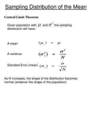
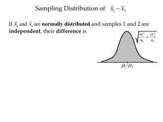
Sampling Distribution of If and are normallydistributed and samples 1 and 2 are independent, their difference is
Sampling Distribution of If and are normallydistributed and samples 1 and 2 are independent, their difference is The normal distribution is not used if s1 and s2 are unknown. The t-distribution is used instead with
Sampling Distribution of If and are normallydistributed and samples 1 and 2 are independent, their difference is n1(1 -p1) > 5 n1p1> 5 n2(1 -p2) > 5 n2p2> 5 The sample proportions are pooled (averaged) when testing the equality of proportions.
Sampling Distribution of If and are normallydistributed and samples 1 and 2 are independent, their difference is The sample proportions are pooled (averaged) when testing whether the proportions are equal or not.
Interval estimate of Example 1 Par, Inc. is a manufacturer of golf equipment and has developed a new golf ball that has been designed to provide “extra distance.” In a test of driving distance using a mechanical driving device, a sample of Par golf balls was compared with a sample of golf balls made by Rap, Ltd., a competitor. The sample statistics appear on the next slide.
x1-x2 = 275 – 258 = 17 Interval estimate of Example 1 Sample #1 Par, Inc. Sample #2 Rap, Ltd. Sample Size 120 balls 80 balls Sample Mean 275 yards 258 yards Based on data from previous driving distance tests, the two population standard deviations are 15 and 20 yards, respectively. Develop a 95% confidence interval estimate of the difference between the mean driving distances of the two brands of golf balls.
Interval estimate of Example 1 17 +5.14 yards 11.86 yards to 22.14 yards We are 95% confident that the difference between the mean driving distances of Par and Rap golf balls is between 11.86 to 22.14 yards.
= x1 – x2 Interval estimate of Example 2 Specific Motors of Detroit has developed the M car. 24 M cars and 28 J cars (from Japan) were road tested to compare miles-per-gallon (MPG) performance. The sample statistics are given below. Develop a 90% confidence interval estimate of the difference between the MPG performances of the two models of automobile. M Cars J Cars n 24 cars 28 cars x 29.8 mpg 27.3 mpg s 2.56mpg 1.81 mpg Point estimate of 1-2 = 29.8 – 27.3 = 2.5 MPG
Interval estimate of Example 2 The degrees of freedom are: 40 a = .1000 With 1-a= .9000 a/2 = .0500 (the column of t-table) 40 df = (the row of t-table) t.0500 = 1.684 -t.0500 = -1.684
Interval estimate of Example 2 2.5+ 1.051 1.448 to 3.552 mpg We are 90% confident that the difference between the MPG performances of M cars and J cars is 1.448 to 3.552 mpg
Interval estimate of Example 3 Market Research Associates is conducting research to evaluate the effectiveness of a client’s new advertising campaign. Before the new campaign began, a telephone survey of 150 households in the test market area showed 60 households “aware” of the client’s product. The new campaign has been initiated with TV and newspaper advertisements running for three weeks. A survey conducted immediately after the new campaign showed 120 of 250 households “aware” of the client’s product. Develop a 95% confidence interval estimate of the difference between the proportion of households that are aware of the client’s product.
Interval estimate of Example 3 z.0250= 1.96 a = .0500 a/2 = .0250 1-a= .9500 .08 + .10 We are 95% confident that the “change in awareness” due to the campaign is between -0.02 and 0.18…
Hypothesis Tests Aboutm1-m2 Example 1 (continued) Can we conclude, using a 5% level of significance, that the mean driving distance of Par, Inc. golf balls is greater than the mean driving distance of Rap, Ltd. golf balls? 1. Develop the hypotheses. H0: 1– 2<0 Ha: 1 –2 > 0
Hypothesis Tests Aboutm1-m2 • Determine the critical value z.0500 = 1.645 a / 1 = .0500 a = .0500 3. Compute the value of the test statistic.
Hypothesis Tests Aboutm1-m2 4. Reject or do not reject the null hypothesis Do Not Reject H0 Reject H0 z 0 6.49z-stat 1.645 At the 5% level of significance, the sample evidence indicates the mean driving distance of Par, Inc. golf balls is greater than the mean driving distance of Rap, Ltd. golf balls.
Hypothesis Tests Aboutm1-m2 Example 2 (continued) Can we conclude, using a 5% level of significance, that the miles-per-gallon (MPG) performance of M cars is greater than the MPG performance of J cars? M Cars J Cars Recall n 24 cars 28 cars x 29.8 mpg 27.3 mpg s 2.56mpg 1.81 mpg H0: 1 - 2<0 1. Develop the hypotheses. Ha: 1 - 2 > 0
Hypothesis Tests Aboutm1-m2 2. Determine the critical value. (column) a /1 = .050 t.050= 1.684 df = 40 (row) 3. Compute the value of the test statistic.
Hypothesis Tests Aboutm1-m2 4. Reject or do not reject the null hypothesis At 5% significance, fuel economy of M cars is greater than the mean fuel economy of J cars. Do Not Reject H0 Reject H0 t 0 4.003 t-stat 1.684t050
Hypothesis Tests Aboutp1-p2 Example 3 (continued) Can we conclude, using a 5% level of significance, that the proportion of households aware of the client’s product increased after the new advertising campaign? 1. Develop the hypotheses. H0: p1-p2<0 Ha: p1-p2 > 0 z.05 = 1.645 a = .0500 2. Determine the critical value. 3. Compute the value of the test statistic.
Hypothesis Tests Aboutp1-p2 4. Reject or do not reject the null hypothesis Do Not Reject H0 Reject H0 z 1.645 1.57 z-stat 0 z.050 We cannot conclude that the proportion of households aware of the client’s product increased after the new campaign.
Hypothesis Tests Aboutp1-p2 Example 4 John is a political candidate who wants to know if female support for his candidacy is the same as his male support using a 5% level of significance. A survey conducted shows 310 of 620 females surveyed said they will vote for John while the same survey said 362 of 680 males said they will vote for John. 1. Develop the hypotheses. H0: p1-p2 = 0 Ha: p1-p2≠0
Hypothesis Tests Aboutp1-p2 2. Determine the critical value. ±z.0250 = ±1.96 a / 2 = .0250 a = .0500 3. Compute the value of the test statistic.
Hypothesis Tests Aboutp1-p2 4. Reject or do not reject the null hypothesis 1 – a = .9700 Reject H0 Do Not Reject H0 Reject H0 0 -1.96 1.96 -1.15z-stat We cannot conclude that support from female voters is different from support from male voters.
Matched Samples Example: Express Deliveries A Chicago-based firm has documents that must be quickly distributed to district offices throughout the U.S. The firm must decide between two delivery services, UPX (United Parcel Express) and INTEX (International Express), to transport its documents. In testing the delivery times of the two services, the firm sent two reports to a random sample of its district offices with one report carried by UPX and the other report carried by INTEX. Do the data on the next slide indicate a difference in mean delivery times for the two services? Use a 5% level of significance.
Matched Samples Delivery Time (Hours) District Office UPX INTEX Difference (d) 1 2 3 -1 2 -2 5 32 30 19 16 15 18 14 10 7 16 25 24 15 15 13 15 15 8 9 11 7 4 6 Seattle Los Angeles Boston Cleveland New York Houston Atlanta St. Louis Milwaukee Denver Sum = 27
Matched Samples 4.3 3.3 1.3 -1.7 -0.7 0.3 -3.7 -0.7 -4.7 2.3 7 6 4 1 2 3 -1 2 -2 5 7– 2.7 6 – 2.7 4 – 2.7 1 – 2.7 2 – 2.7 3 – 2.7 -1 – 2.7 2 – 2.7 -2 – 2.7 5 – 2.7 18.49 10.89 1.69 2.89 0.49 0.09 13.69 0.49 22.09 5.29 76.1 Sum = sd = 2 8.5 sd= 2.9
Matched Samples with d = m1 – m2 1. Develop the hypotheses Ha: d H0: d = 0 No difference exists Adifference exists a = .050. 2. Determine the critical values with Since this is a two-tailed test (the column of the t-table) a /2 = .025 (the row of the t-table) df = 10 – 1 = 9 - t.025 = -2.262 t.025 = 2.262 3. Compute the value of the test statistic.
Matched Samples 4. Reject or do not reject the null hypothesis Reject H0 Do Not Reject Reject H0 H0: d = 0 -2.262 2.262-t.025t.025 0 2.94 t-stat At the 5% level of significance, the sample evidence indicates there is a difference in mean delivery times for the two services.