A sampling distribution lists the possible values of a statistic (e.g., sample mean or sample proportion) and their pro

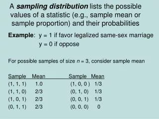
1. A sampling distributionlists the possible values of a statistic (e.g., sample mean or sample proportion) and their probabilities Example: y = 1 if favor legalized same-sex marriage y = 0 if oppose For possible samples of size n = 3, consider sample mean Sample Mean Sample Mean (1, 1, 1) 1.0 (1, 0, 0 ) 1/3 (1, 1, 0) 2/3 (0, 1, 0) 1/3 (1, 0, 1) 2/3 (0, 0, 1) 1/3 (0, 1, 1) 2/3 (0, 0, 0) 0

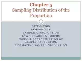
2. Sampling distribution of a statistic is the probability distribution for the possible values of the statistic Ex. Suppose P(0) = P(1) = ½. For random sample of size n = 3, each of 8 possible samples is equally likely. Sampling distribution of sample proportion is Sample proportion Probability 0 1/8 1/3 3/8 2/3 3/8 1 1/8

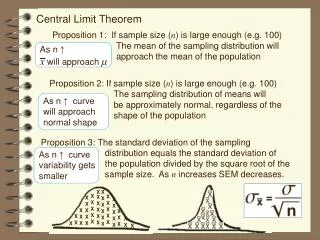
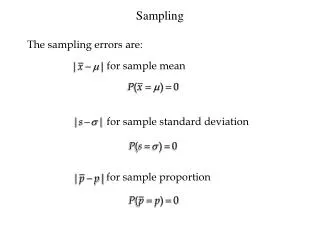
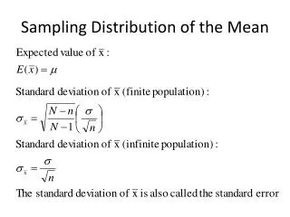
3. Sampling distribution of sample mean • is a variable, its value varying from sample to sample about the population mean µ • Standard deviation of sampling distribution of is called the standard error of • For random sampling, the sampling distribution of has mean µ and standard error

4. Example: For binary data (y =1 or 0) with P(Y=1) =  (with 0 <  < 1), one can show that When  = 0.50, then = 0.50, and standard error is • n standard error • .289 • 100 .050 • 200 .035 • 1000 .016

5. Note standard error goes down as n goes up (i.e., tends to fall closer to µ) • With n = 1000, standard error = 0.016, so if the sampling distribution is bell-shaped, with very high probability the sample proportion falls within 3(0.016) = 0.05 of population proportion of 0.50 (i.e., between about 0.45 and 0.55) • Number of timesy = 1 (i.e., number of people in favor) is 1000 x (proportion), so that the “count” variable has • mean = 1000x(0.50) = 500 • std. dev. 1000x(0.016) = 16

6. Practical implication: This chapter presents theoretical results about spread (and shape) of sampling distributions, but it implies how different studies on the same topic can vary from study to study in practice (and therefore how precise any one study will tend to be) Ex. You plan to sample 1000 people to estimate the population proportion supporting Obama’s health care plan. Other people could be doing the same thing. How will the results vary among studies (and how precise are your results)? The sampling distribution of the sample proportion in favor of the health care plan has standard error describing the likely variability from study to study.

7. Ex. Many studies each take sample of n = 1000 to estimate population proportion • We’ve seen the sample proportion vary from study to study around 0.50 with standard error = 0.016, when π=0,5 • Flipping a coin 1000 times simulates the process when the population proportion = 0.50.

8. Central Limit Theorem: For random sampling with “large” n, the sampling dist. of the sample mean is approximately a normal distribution • Approximate normality applies no matter what the shape of the population dist. (Figure, next page) • How “large” n needs to be depends on skew of population distribution, but usually n ≥ 30 sufficient

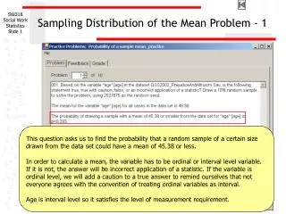
10. Example: You plan to randomly sample 100 ITU students to estimate population proportion who have a part time job. Find the probability that your sample proportion falls within 0.04 of population proportion, if that population proportion = 0.30(i.e., between 0.26 and 0.34) y = 1, yes y = 0, no µ = = 0.30, By CLT, sampling distribution of sample mean (which is the proportion “yes”) is approx. normal with mean 0.30, standard error

11. 0.26 has z-score z = (0.26 - 0.30)/0.0458 = -0.87 • 0.34 has z-score z = (0.34 - 0.30)/0.0458 = 0.87 • P(sample mean ≥ 0.34) = 0.19 • P(sample mean ≤ 0.26) = 0.19 • P(0.26 ≤ sample mean ≤ 0.34) = 1 – 2(0.19) = 0.62 The probability is 0.62 that the sample proportion will fall within 0.04 of the population proportion How would this change if n is larger (e.g., 200)?

12. Some Summary Comments • Consequence of CLT: When the value of a variable is a result of averaging many individual influences, no one dominating, the distribution is approx. normal (e.g., IQ, blood pressure) • In practice, we don’t know µ, but we can use spread of sampling distribution as basis of inference for unknown parameter value • We have now discussed three types of distributions:

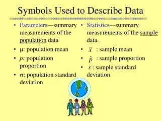
13. Population distribution – described by parameters such as µ, σ (usually unknown) • Sample data distribution – described by sample statistics such as sample mean , standard deviation s • Sampling distribution – probability distribution for possible values of a sample statistic; determines probability that statistic falls within certain distance of population parameter (graphic showing differences)

14. Ex. (categorical): Poll about health care Statistic = sample proportion favoring the new health care plan What is (1) population distribution, (2) sample distribution, (3) sampling distribution? Ex. (quantitative): Experiment about impact of cell-phone use on reaction times Statistic = sample mean reaction time What is (1) population distribution, (2) sample distribution, (3) sampling distribution?

15. By the Central Limit Theorem (multiple choice) • All variables have approximately normal sample data distributions if a random sample has at least 30 observations • Population distributions are normal whenever the population size is large (at least about 30) • For large random samples, the sampling distribution of the sample mean is approximately normal, regardless of the shape of the population distribution • The sampling distribution looks more like the population distribution as the sample size increases • All of the above