Download
1 / 246
2.46k likes | 2.6k Vues
IE341: Introduction to Design of Experiments. Last term we talked about testing the difference between two independent means. For means from a normal population, the test statistic is

E N D
Last term we talked about testing the difference between two independent means. For means from a normal population, the test statistic is where the denominator is the estimated standard deviation of the difference between two independent means. This denominator represents the random variation to be expected with two different samples. Only if the difference between the sample means is much greater than the expected random variation do we declare the means different.
We also covered the case where the two means are not independent, and what we must do to account for the fact that they are dependent.
And finally, we talked about the difference between two variances, where we used the F ratio. The F distribution is a ratio of two chi-square variables. So if s21 and s22 possess independent chi-square distributions with v1 and v2 df, respectively, then has the F distribution with v1 and v2 df.
All of this is valuable if we are testing only two means. But what if we want to test to see if there is a difference among three means, or four, or ten? What if we want to know whether fertilizer A or fertilizer B or fertilizer C is best? In this case, fertilizer is called a factor, which is the condition under test. A, B, C, the three types of fertilizer under test, are called levels of the factor fertilizer. Or what if we want to know if treatment A or treatment B or treatment C or treatment D is best? In this case, treatment is called a factor. A,B,C,D, the four types of treatment under test, are called levels of the factor treatment. It should be noted that the factor may be quantitative or qualitative.
Enter the analysis of variance! ANOVA, as it is usually called, is a way to test the differences between means in such situations. Previously, we tested single-factor experiments with only two treatment levels. These experiments are called single-factor because there is only one factor under test. Single-factor experiments are more commonly called one-way experiments. Now we move to single-factor experiments with more than two treatment levels.
Let’s start with some notation. Yij = ith observation in the jth level N = total number of experimental observations = the grand mean of all N experimental observations = the mean of the observations in the jth level nj = number of observations in the jth level; the nj are called replicates. Replication of the design refers to using more than one experimental unit for each level. If there are the same number n replicates for each treatment, the design is said to be balanced.
Designs are more powerful if they are balanced, but balance is not always possible. Suppose you are doing an experiment and the equipment breaks down on one of the tests. Now, not by design but by circumstance, you have unequal numbers of replicates for the levels. In all the formulas, we used nj as the number of replicates in treatment j, notn, so there is no problem.
Notation continued = the effect of the jth level J = number of treatment levels eij = the “error” associated with the ith observation in the jth level, assumed to be independent normally distributed random variables with mean = 0 and variance = σ2, which are constant for all levels of the factor.
For all experiments, randomization is critical. So to draw any conclusions from the experiment, we must require that the treatments be applied in random order. We must also assign the experimental units to the treatments randomly. If all this randomization occurs, the design is called a completely randomized design.
This model is for a one-way or single-factor ANOVA. The goal of the model is to test hypotheses about the treatment effects and to estimate them. If the treatments have been selected by the experimenter, the model is called a fixed-effects model. In this case, the conclusions will apply only to the treatments under consideration.
Another type of model is the random effects model or components of variance model. In this situation, the treatments used are a random sample from large population of treatments. Here the τi are random variables and we are interested in their variability, not in the differences among the means being tested.
First, we will talk about fixed effects, completely randomized, balanced models. In the model we showed earlier, the τj are defined as deviations from the grand mean so It follows that the mean of the jth treatment is
Now the hypothesis under test is: Ho: μ1= μ2 = μ3 = … μJ Ha: μj≠ μk for at least one j,k pair The test procedure is ANOVA, which is a decomposition of the total sum of squares into its components parts according to the model.
The total SS is and ANOVA is about dividing it into its component parts. SS= variability of the differences among the J levels SSε = pooled variability of the random error within levels
This is easy to see because But the cross-product term vanishes because
So SStotal = SS treatments + SS error Most of the time, this is called SStotal = SS between + SS within Each of these terms becomes an MS (mean square) term when divided by the appropriate df.
The df for SSerror = N-J because and the df for SSbetween = J-1 because there are J levels.
Now the expected values of each of these terms are E(MSerror) = σ2 E(MStreatments) =
Now if there are no differences among the treatment means, then for all j. So we can test for differences with our old friend F with J -1 and N -J df. Under Ho, both numerator and denominator are estimates of σ2 so the result will not be significant. Under Ha, the result should be significant because the numerator is estimating the treatment effects as well as σ2.
The results of an ANOVA are presented in an ANOVA table. For this one-way, fixed-effects, balanced model: Source SS df MS p Model SSbetweenJ-1 MSbetween p Error SSwithin N-J MSwithin Total SStotal N-1
Let’s look at a simple example. A product engineer is investigating the tensile strength of a synthetic fiber to make men’s shirts. He knows from prior experience that the strength is affected by the weight percent of cotton in the material. He also knows that the percent should range between 10% and 40% so that the shirts can receive permanent press treatment.
The engineer decides to test 5 levels: 15%, 20%, 25%, 30%, 35% and to have 5 replicates in this design. His data are
In this tensile strength example, the ANOVA table is In this case, we would reject Ho and declare that there is an effect of the cotton weight percent. Source SS df MS p Model 475.76 4 118.94<0.01 Error 161.20 20 8.06 Total 636.96 24
We can estimate the treatment parameters by subtracting the grand mean from the treatment means. In this example, τ1 = 9.80 – 15.04 = -5.24 τ2 = 15.40 – 15.04 = +0.36 τ3 = 17.60 – 15.04 = -2.56 τ4 = 21.60 – 15.04 = +6.56 τ5 = 10.80 – 15.04 = -4.24 Clearly, treatment 4 is the best because it provides the greatest tensile strength.
Now you could have computed these values from the raw data yourself instead of doing the ANOVA. You would get the same results, but you wouldn’t know if treatment 4 was significantly better. But if you did a scatter diagram of the original data, you would see that treatment 4 was best, with no analysis whatsoever. In fact, you should always look at the original data to see if the results do make sense. A scatter diagram of the raw data usually tells as much as any analysis can.
How do you test the adequacy of the model? The model assumes certain assumptions that must hold for the ANOVA to be useful. Most importantly, that the errors are distributed normally and independently. The error for each observation, sometimes called the residual, is
A residual check is very important for testing for nonconstant variance. The residuals should be structureless, that is, they should have no pattern whatsoever, which, in this case, they do not.
These residuals show no extreme differences in variation because they all have about the same spread. They also do not show the presence of any outlier. An outlier is a residual value that is vey much larger than any of the others. The presence of an outlier can seriously jeopardize the ANOVA, so if one is found, its cause should be carefully investigated.
A histogram of residuals shows the distribution is slightly skewed. Small departures from symmetry are of less concern than heavy tails.
Another check is for normality. If we do a normal probability plot of the residuals, we can see whether normality holds.
A normal probability plot is made with ascending ordered residuals on the x-axis and their cumulative probability points, 100(k-.5)/n, on the y-axis. k is the order of the residual and n = number of residuals. There is no evidence of an outlier here. The previous slide is not exactly a normal probability plot because the y-axis is not scaled properly. But it does gives a pretty good suggestion of linearity.
A plot of residuals vs run order is useful to detect correlation between the residuals, a violation of the independence assumption. Runs of positive or of negative residuals indicates correlation. None is observed here.
One of the goals of the analysis is to estimate the level means. If the results of the ANOVA shows that the factor is significant, we know that at least one of the means stands out from the rest. But which one or ones? The procedures for making these mean comparisons are called multiple comparison methods. These methods use linear combinations called contrasts.
A contrast is a particular linear combination of level means, such as to test the difference between level 4 and level 5. Or if one wished to test the average of levels 1 and 3 vs levels 4 and 5, he would use . In general, where
An important case of contrasts is called orthogonal contrasts. Two contrasts in a design with coefficients cj and dj are orthogonal if
There are many ways to choose the orthogonal contrast coefficients for a set of levels. For example, if level 1 is a control and levels 2 and 3 are two real treatments, a logical choice is to compare the average of the two treatments with the control: and then the two treatments against one another: These two contrasts are orthogonal because
Only J-1 orthogonal contrasts may be chosen because the J levels have only J-1 df. So for only three levels, the contrasts chosen exhaust those available for this experiment. Contrasts must be chosen before seeing the data so that experimenters aren’t tempted to contrast the levels with the greatest differences.
For the tensile strength experiment with 5 levels and thus 4 df, the 4 contrasts are: C1= 0(5)(9.8)+0(5)(15.4)+0(5)(17.6)-1(5)(21.6)+1(5)(10.8) =-54 C2= +1(5)(9.8)+0(5)(15.4)+1(5)(17.6)-1(5)(21.6)-1(5)(10.8) =-25 C3= +1(5)(9.8)+0(5)(15.4)-1(5)(17.6)+0(5)(21.6)+0(5)(10.8) =-39 C4= -1(5)(9.8)+4(5)(15.4)-1(5)(17.6)-1(5)(21.6)-1(5)(10.8) = 9 These 4 contrasts completely partition the SStreatments. Then the SS for each contrast is formed:
Now the revised ANOVA table is Source SS df MS p Weight % 475.76 4 118.94 <0.001 C1 291.60 1 291.60 <0.001 C2 31.25 1 31.25 <0.06 C3 152.10 1 152.10 <0.001 C4 0.81 1 0.81 <0.76 Error 161.20 20 8.06 Total 636.96 24
So contrast 1 (level 5 – level 4) and contrast 3 (level 1 – level 3) are significant. Although the orthogonal contrast approach is widely used, the experimenter may not know in advance which levels to test or they may be interested in more than L-1 comparisons. A number of other methods are available for such testing.
These methods include: Scheffe’s Method Least Significant Difference Method Duncan’s Multiple Range Test Newman-Keuls test There is some disagreement about which is the best method, but it is best if all are applied only after there is significance in the overall F test.
Now let’s look at the random effects model. Suppose there is a factor of interest with an extremely large number of levels. If the experimenter selects L of these levels at random, we have a random effects model or a components of variance model.
The linear statistical model is as before, except that both and are random variables instead of simply . Because and are independent, the variance of any observation is These two variances are called variance components, hence the name of the model.
The requirements of this model are that the are NID(0,σ2), as before, and that the are NID(0, ) and that and are independent. The normality assumption is not required in the random effects model. As before, SSTotal = SStreatments + SSerror And the E(MSerror) = σ2. But now E(MStreatments) = σ2 + n So the estimate of is
The computations and the ANOVA table are the same as before, but the conclusions are quite different. Let’s look at an example. A textile company uses a large number of looms. The process engineer suspects that the looms are of different strength, and selects 4 looms at random to investigate this.
The results of the experiment are shown in the table below. The ANOVA table is Source SS df MS p Looms 89.19 3 29.73 <0.001 Error 22.75 12 1.90 Total 111.94 15