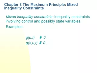
Chapter 3 The Maximum Principle: Mixed Inequality Constraints
630 likes | 1.25k Vues
Mixed inequality constraints: Inequality constraints involving control and possibly state variables. Examples: g(u,t) 0 , g(x,u,t) 0 . Chapter 3 The Maximum Principle: Mixed Inequality Constraints. 3.1 A Maximum Principle for Problems with Mixed Inequality Constraints.

Chapter 3 The Maximum Principle: Mixed Inequality Constraints
E N D
Presentation Transcript
Mixed inequality constraints: Inequality constraints involving control and possibly state variables. Examples: g(u,t) 0 , g(x,u,t) 0 . Chapter 3 The Maximum Principle: Mixed Inequality Constraints
3.1 A Maximum Principle for Problems with Mixed Inequality Constraints • State equation: where x(t) En, u(t) Emand f: En x Em xE1 En is assumed to be continuously differentiable. • Objective function: where F: En x Em x E1 E1, and S: En x E1 E1 are continuously differentiable and T is the terminal time.
u(t), t[0,T] is admissible if it is piecewise continuous and satisfies the mixed constraints. where g: Enx EmxE1 Eq is continuously differentiable and terminal inequality and equality constraints: where a: Enx E1 Ela and b: Enx E1 Elbare continuously differentiable.
Interesting case of the terminal inequality constraint: where Y is a convex set, X is the reachableset from the initial state x0, i.e., Notes:(i) (3.6) does not depend explicitly on T. (ii) Feasible set defined by (3.4) and (3.5) need not be convex. (iii) (3.6) may not be expressible by a simple set of inequalities.
Full rank or constraint qualifications condition holds for all arguments x(t), u(t), t, t[0,T], and hold for all possible values of x(T) and T. • Hamiltonian function H: Enx Emx En x E1 E1is where En(a row vector).
Lagrangian function L: Enx Emx Enx Eqx E1 E1 is where Eqis a row vector, whose components are called Lagrange multipliers. • Lagrange multipliers satisfy the complimentary slackness conditions:
The adjoint vector satisfies the differential equation • with the boundary conditions where Elaand Elbare constant vectors. • The necessary conditions for u* by the maximum principle are that there exist , , , such that (3.11) holds, i.e.,
Special Case: In the case of terminal constraint (3.6), the terminal conditions on the state and the adjoint variables in (3.11) will be, respectively, Furthermore, if the terminal time T in (3.1)-(3.5) is unspecified, there is an additional necessary transversality condition for T* to be optimal if T*(0,) .
Remark 3.1: We should have H=0F+f in (3.7) with 0 0. However, we can set 0=1 in most applications Remark 3.2:If the set Y in (3.6) consists of a single point Y={k}, then as in (2.75), the transversality condition reduces to simply *(T) equals to a constant to be determined, since x*(T)=k. In this case, salvage value function S can be disregarded.
Example 3.1: Consider the problem: subject to Note that constraints (3.16) are of the mixed type (3.3). They can also be rewritten as 0 u x. Solution: The Hamiltonian is so that the optimal control has the form
To get the adjoint equation and the multipliers associated with constraints (3.16), we form the Lagrangian: From this we get the adjoint equation Also note that the optimal control must satisfy and 1 and 2 must satisfy the complementary slackness conditions
It is obvious for this simple problem that u*(t)=x(t) should be the optimal control for all t[0,1]. We now show that this control satisfies all the conditions of the Lagrangian form of the maximum principle. • Since x(0)=1, the control u*= x gives x= etas the solution of (3.15). Because x=et>0, it follows that u*= x > 0; thus 1=0 from (3.20). • From (3.19) we then have 2=1+. Substituting this into (3.18) and solving gives Since the right-hand side of (3.22) is always positive, u*= x satisfies (3.17). Note that 2 = e1-t 0 and x-u* = 0, so (3.21) holds.
3.2 Sufficiency Conditions Let D En be a convexset. A function :D E1is concave, if forall y,z D and for all p[0,1], The function is quasiconcave if (3.23) is relaxed to is strictlyconcave if y z and p (0,1), and (3.23) holds with a strict inequality. is convex, quasiconvex, or strictly convex if - is concave, quasiconcave, or strictly concave, respectively.
Theorem 3.1 Let (x*,u*,,μ,,) satisfy the necessary conditions in (3.11). If H(x,u,(t),t) is concave in (x,u) at each t[0,T], S in (3.2) is concave in x, g in (3.3) is quasiconcave in (x,u), a in (3.4) is quasiconcave in x, and b in (3.5) is linear in x, then (x*,u*) is optimal. The concavity of the Hamiltonian with respect to (x,u) is a crucial condition in Theorem 3.1. So we replace the concavity requirement on the Hamiltonian in Theorem 3.1 by a concavity requirement on H0, where
Theorem 3.2 Theorem 3.1 remains valid if and, if in addition, we drop the quasiconcavity requirement on g and replace the concavity requirement on H in Theorem 3.1 by the following assumption:For each t[0,T], if we define A1(t)= {x|u, g(x,u,t) 0 for some u}, then H0(x,(t),t) is concave on A1(t), if A1(t) is convex.If A1(t) is not convex,we assume that H0 has a concave extension to co(A1(t)), the convex hull of A1(t).
3.3 Current-Value Formulation Assume a constant continuous discount rate 0. The time dependence in (3.2) comes only through the discount factor. The objective is to subject to (3.1) and (3.3)-(3.5).
The standard Hamiltonian is and the standard Lagrangian is with sand s and ssatisfying
The current-value Hamiltonian is defined as and the current-value Lagrangian • We define we can rewrite (3.27) and (3.28) as From (3.35), we have and then from (3.29)
where (T) follows immediately from terminal conditions for s(T) in (3.30) and (3.36) • The complementary slackness conditions satisfied by the current-value Lagrange multipliers and are on account of (3.31), (3.32), (3.35), and (3.39). • From (3.14), the necessary transversality condition for T* to be optimal is:
Special Case: When the terminal constraints is given by (3.6) instead of (3.4) and (3.5), we need to replace the terminal condition on the state and the adjoint variables, respectively, by (3.12) and Example 3.2:Use the current-value maximum principle to solve the following consumption problem for = r: subject to the wealth dynamics where W0>0. Note that the condition W(T) = 0 is sufficient to make W(t) 0 for all t. We can interpret lnC(t) as the utility of consuming at the rate C(t) per unit time at time t.
Solution: The current-value Hamiltonian formulation: where the adjoint equation is since we assume = r, and where is some constant to be determined. The solution of (3.44) is simply (t)= for 0t T.
To find the optimal control, we maximize H by differentiating (3.43) with respect to C and setting the result to zero: which implies C=1/=1/. Using this consumption level in the wealth dynamics gives which can be solved as
Setting W(T)=0 gives Therefore, the optimal consumption since = r.
3.4 Terminal Conditions/Transversality Conditions Case 1:Free-end point. In this case x(T) X. From (3.11), it is obvious that for the free-end-point problem if (x)0, then (T)=0. Case 2: Fixed-end point. In this case, the terminal condition is and the transversality condition in (3.11) does not provide any information for (T). *(T) will be some constant .
Case 3: One-sided constraints. In this case, the ending value of the state variable is in a one-sided interval where k X. In this case it is possible to show that and Case 4: A general case. A general ending condition is
Example 3.3 Consider the problem subject to Solution: The Hamiltonian is The optimal control has the form
The adjoint equation is with the transversality conditions Since (t) is monotonically increasing, the control (3.51) can switch at most once, and it can only switch from u* = -1 to u* = 1. Let the switching time be t* 2. The optimal control is Since the control switches at t*, (t*) must be 0. Solving (3.52) we get
There are two cases t* < 2 and t* = 2. We analyze the first case first. Here (2)=2-t* > 0; therefore from (3.53), x(2) = 0. Solving for x with u* given in (3.54), we obtain which makes t*=3/2. Since this satisfies t* < 2, we do not have to deal with the case t*= 2.
Isoperimetric or budget constraint: It is of the form where l: En x Em x E1 E1is assumed nonnegative,bounded,and continuously differentiable and K is a positive constant representing the amount of the budget. It can be converted into a one-sided constraint by the state equation
3.4.1 Examples Illustrating Terminal Conditions Example 3.4: The problem is: where B is a positive constant. Solution: The Hamiltonian for the problem is given in (3.43) and the adjoint equation is given in (3.44) except that the transversality conditions are from Row 3 of Table 3.1:
In Example 3.2 the value of , the terminal value of (T), was We now have two cases: (i) B and (ii) < B. • In case (i), the solution of the problem is the same as that of Example 3.2, because by setting (T)= and recalling that W(T) = 0 in that example, it follows that (3.59) holds. • In case (ii), we set (T)= B and use (3.44) which is = 0. Hence (t)= B for all t. The Hamiltonian maximizing condition remains unchanged. Therefore, the optimal consumption is C=1/ =1/B
Solving (3.58) with this C gives It is easy to show that is nonnegative since < B. Note that (3.59) holds for case (ii).
Example 3.5: A Time-Optimal Control Problem. Consider a subway train of mass m (assume m=1), which moves along a smooth horizontal track with negligible friction. The position x of the train along the track at time t is determined by Newton’s Law of Motion
Solution: The standard Hamiltonian function is: where the adjoint variables 1 and 2 satisfyThus, 1 =c1, 2 = c2 + c1 (T- t).
The Hamiltonian maximizing condition yields the form of the optimal control to be which together with the bang-bang control policy (3.64) implies either The transversality condition (3.14) with y(T) = 0 and S 0 yields
We can put - and+ intoa singleswitching curve as If the initial state (x0,y0) lies on the switching curve, then we have u*= +1(resp., u*= -1) if x0 0 (resp., x0<0); i.e, if (x0,y0) lies on + (resp.,- ). If the initial state (x0,y0) is not on the switching curve, then we choose, between u*= 1 and u*= -1, that which moves the system toward the switching curve. By inspection, it is obvious that above the switching curve we must choose u*= -1 and below we must choose u*= +1.
Figure 3.2: Minimum Time Optimal Response for Problem (3.63)
The other curves in Figure 3.2 are solutions of the differential equations starting from initial points (x0,y0). If (x0,y0) lies above the switching curve as shown in Figure 3.2, we use u* = -1 to compute the curve as follows:Integrating these equations givesElimination of t between these two gives
This is the equation of the parabola in Figure 3.2 through (x0,y0) . The point of intersection of the curve (3.66) with the switching curve + is obtained by solving (3.66) and the equation for +, namely 2x = y2, simultaneously, which gives where the minus sign in the expression for y* in (3.67) was chosen since the intersection occurs when y* is negative. The time t* to reach the switching curve, called the switching time, given that we start above it, is
To find the minimum total time to go from the starting point (x0,y0) to the origin (0,0), we substitute t* into the equation for + in Column (b) of Table 3.2; this gives • As a numerical example, start at the point (1.1). Then the equation of the parabola (3.66) is 2x = 3- y2 . The switching point (3.67) is . Finally, the switching time is t*= from (3.68). Substituting into (3.69), we find the minimum time to stop is T=
To complete the solution of this numerical example let us evaluate c1 and c2, which are needed to obtain 1and 2. Since (1,1) is above the switching curve, u*(T)= 1 and therefore, c2 = 1. To complete c1, we observe that c2 + c1(T-t*) = 0 so that • In exercises 3.14-3.17, you are asked to work other examples with different starting points above, below, and on the switching curve. Note that t*= 0 by definition, if the starting point is on the switching curve.
3.5 Infinite Horizon and Stationarity • Transversality Conditions Free-end problem: one-side constraint: • Stationarity Assumption:
Long-run stationary equilibrium It is defined by the quadruple satisfying • Clearly, if the initial condition the optimal control is for all t. • If the constraint involving g is not imposed, may be dropped from the quadruple. In this case, the equilibrium is defined by the triple satisfying
Example 3.6:Consider the problem: subject to Solution: By (3.73) we set where is a constant to be determined. This gives the optimal control , and setting , we see all the conditions of (3.73) hold, including the Hamiltonian maximizing condition.
Furthermore andW = W0satisfy the transversality conditions (3.71). Therefore, by the sufficiency theorem, the control obtained is optimal. Note that the interpretation of the solution is that the trust spends only the interest from its endowment W0. Note further that the triple is an optimal long-run stationary equilibrium for the problem.