Maximum Modulus Principle:
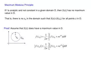
Maximum Modulus Principle: If f is analytic and not constant in a given domain D, then |f(z)| has no maximum value in D. That is, there is no z 0 in the domain such that |f(z)| |f(z 0 )| for all points z in D. Proof: Assume that |f(z)| does have a maximum value in D. R. z 0. C R.

Maximum Modulus Principle:
E N D
Presentation Transcript
Maximum Modulus Principle: If f is analytic and not constant in a given domain D, then |f(z)| has no maximum value in D. That is, there is no z0 in the domain such that |f(z)||f(z0)| for all points z in D. Proof: Assume that |f(z)| does have a maximum value in D. R z0 CR
Alternatively Theorem: If f is analytic, continuous and not constant in a closed bounded region D, then the maximum value of |f(z)| is achieved only on the boundary of D. Some other aspects of the maximum modulus theorem: Assume that f(z) is not 0 in a region R. Then if f(z) is analytic in R, then so is 1/f(z). Result: minimum of |f(z)| also occurs on the boundary. Since the max and min of |f(z)| are on the boundary, so is the max and min of u(x,y). Same applies to v(x,y).
Indented Contour • The complex functions f(z) = P(z)/Q(z) of the improper integrals (2) and (3) did not have poles on the real axis. When f(z) has a pole at z = c, where c is a real number, we must use the indented contour as in Fig 19.13.
THEOREM 19.17 Suppose f has a simple pole z = c on the real axis. If Cr is the contour defined by Behavior of Integral as r →
THEOREM 19.17 proof ProofSince f has a simple pole at z = c, its Laurent series is f(z) = a-1/(z – c) + g(z)where a-1 = Res(f(z), c) and g is analytic at c. Using the Laurent series and the parameterization of Cr,we have (12)
THEOREM 19.17 proof First we see Next, g is analytic at c and so it is continuous at c and is bounded in a neighborhood of the point; that is, there exists an M > 0 for which |g(c + rei)| M. Hence It follows that limr0|I2| = 0 and limr0I2= 0.We complete the proof.
Example 5 Evaluate the Cauchy principal value of Solution Since the integral is of form (3), we consider the contour integral
Fig 19.14 f(z) has simple poles at z = 0 and z = 1 + i in the upper half-plane. See Fig 19.14.
Example 5 (2) • Now we have (13)Taking the limits in (13) as R and r 0, from Theorem 19.16 and 19.17, we have
Example 5 (3) Now Therefore,
Example 5 (4) Using e-1+i = e-1(cos 1 + i sin 1), then
Indented Paths Cr r x0
CR Cr I2 I1
CR Cr I2 I1
Contour Integration Example The graphical interpretation
>> x=[-10*pi:0.1:10*pi]; >> plot(x,sin(x)./x) >> grid on >> axis([-10*pi 10*pi -0.4 1])
>> x=[-10*pi:0.1:10*pi]; >> plot3(x,zeros(size(x)),sin(x)./x) >> grid on >> axis([-10*pi 10*pi -1 1 -0.4 1])
>> x=[-10*pi:0.1:10*pi]; >> y = [-3:0.1:3].'; >> z=ones(size(y))*x+i.*(y*ones(size(x))); >> mesh(x,y,cos(z)./z) >> mesh(x,y,sin(z)./z)
Cauchy’s Inequality: If f is analytic inside and on CR and M is the maximum value of f on CR, then R z0 CR Proof:
As R goes to infinity, then f’(z) must go to zero, everywhere. Then f(z) must be constant. Liouville’s Theorem: If f is entire and bounded in the complex plane, then f(z) is constant throughout the plane. Gauss’s Mean Value Theorem: If f is analytic within and on a given circle, its value at the center is the arithmetic mean of its values on the circle. Proof:
C1 The integral does not go to zero on the circle, the integral can’t be solved this way.
Jordan’s Lemma y x
C1 C2