Download
1 / 12
120 likes | 140 Vues
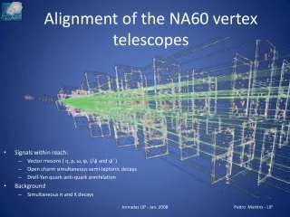
This study focuses on the alignment of the NA60 vertex telescopes to improve the dimuon mass resolution. The signals within reach include vector mesons, open charm simultaneous semi-leptonic decays, Drell-Yan quark-antiquark annihilation, and simultaneous pi and K decays. The study aims to reduce combinatorial background and accurately determine the origin of muons.

E N D
Alignment of the NA60 vertex telescopes • Signals within reach: • Vector mesons ( η, ρ, ω, ϕ, J/ψ and ψ’ ) • Open charm simultaneous semi-leptonic decays • Drell-Yan quark anti-quark annihilation • Background • Simultaneous π and K decays Jornadas LIP - Jan. 2008
muon trigger and tracking hadron absorber magnetic field or ! Muon Other Measuring dimuons in NA60 2.5 T dipole magnet beam tracker vertex telescope targets Matching in coordinate and momentum space • Improved dimuon mass resolution • Reduced combinatorial background • Origin of muons can be accurately determined Jornadas LIP - Jan. 2008
Vertex Telescope’s detectors • Pixels • ALICE: small 4 chip planes. • ALICE: large 8-chip planes. • 256x32 cells • 12.8x13.6 mm2 active area • Used in all runs of 2003 and 2004 • -Strips • BNL: single (complex) sensor. Used in 2004. • Baby-Atlas: 6-chip planes. Used in 2004@400 GeV. Jornadas LIP - Jan. 2008
Motivation • The microstrips were present in 2004, but we never used them in the data reconstruction. • Due to time and people constraints, the studies which originated physics results were only based on a Vertex Telescope consisting of pixel planes alone. • These detectors, namely the ones based on the BNL chips, are 100% “made in Portugal”. • We couldn’t just let them die silently… • A rough alignment should be enough to allow the usage of the microstrips timing information, which will enhance our pile-up rejection capabilities. Who we are and what are we doing We means: André David, Pedro Martins, Pedro Parracho, Pedro Ramalhete and João Seixas. The LIP group at NA60 is coordinated by João Seixas. So far, we have worked on several projects within the experiment with a bigger emphasis on detector conception (pixels, microstrips), DAQ, DCS and data reconstruction. Currently, the “Pedros” are working on their PhD thesis in charmonia production, D0 production and UPC and photonic interaction. Jornadas LIP - Jan. 2008
Residuals • Residual = extrapolated track position - detected cluster • The “extrapolated track “ comes from the other telescope planes, aligned with a preliminary setup. • The corresponding residuals usually follow a “gaussian” distribution on both transverse directions (each pixel is very small on both directions). • To align a chip we simply subtract the obtained residuals to the chip’s position on the setup file. • Hence, with a peak finder algorithm together with a gaussian fit, we are able to minimize the residuals to zero via 2. • This was used to align the pixel planes in 2003 and 2004. • It looked somewhat disapointing with the strips: Cluster (digits) Pixel residual Extrapolated track In black, coordinates of the center of each strip (digit). With colour, the pixel track distribution extrapolated on the Z coordinates of the plane XY distribution of the residuals for an ATLAS microstrip plane Jornadas LIP - Jan. 2008
Residuals method applied to the microstrips Event display for a BNL strip sensor: each red line is a digit. Notice the non-trivial geometrical arrangement of the strips. Saddly, this method does not work on the strips. • The long dimension of a single strip is not negligible • The method only uses the center of this long strip • The extrapolated tracks on the strip sensors are not homogeneous, need normalization • Since the strips are long, it is possible to have a denser track distribution in one side of the strip, biasing the results • The obtained residual’s distribution was of poor quality. BNL strips Jornadas LIP - Jan. 2008
j i The correlation method • Let’s start partitioning the physical space: • The obtained plots were lacking statistics.. • Pearson product-moment correlation coefficient : Track distribution on the BNL -strip planes Plane 2 – ATLAS -strip plane … and we did something about it! • Where: • v - There is an extrapolated track on a given bin. • w - There is a cluster on that given bin. Jornadas LIP - Jan. 2008
Correlation Map Strips Workaround – several strips as one Correlation Map Strips k Strips Take a strip close to the first one. Change the “universe” coordinates (track hits) to match the first strip coordinates. And the events of the second strip are automatically added to the correlation map. The results were encouraging But there are still some issues Jornadas LIP - Jan. 2008
Problem 1: How to see the “correlation strip” within our correlation map? • We needed something fast and reliable. • Our approach consisted in defining a threshold from which we established a binary map for this correlation map. The chosen strip is there. “Binary map” for plane 4, sensor 1, using a threshold of 0.15 for the previously calculated correlation. Jornadas LIP - Jan. 2008
Problem 2: How to identify the cluster where the strip belongs? • We used the Hoshen-Kopelman technique, which is usually used in percolation studies. • Our map becomes a binary matrix. • We sweep the matrix searching for bins with content=1 and check if they are neighbours with other bins in the same condition. • All the bins in the same neighbourhood become a “cluster”, with a unique label. • There is a final sweep through the matrix to order the labels. Zooming… “ASCII map” for plane 4, sensor 1, using a threshold of 0.15 and after labeling via Hoshen-Kopelman. Jornadas LIP - Jan. 2008
Problem 3: How to calculate the center of the cluster • Many methods can be used, from a simple linear fit to an average of the positions of the cluster’s bins. • For this meeting I’ve calculated the center of the cluster using a very simple average between the X and Y coordinates of the cluster. This is clearly a bad method, a fit will be implemented a.s.a.p. This was only done to show that we are ready to extract the strip coordinates and use them for the plane alignment. Calculated center of the cluster #10 (blue): (x,y) = (0.317, 0.317) PRELIMINARY! “Colour map” for plane 4, sensor 1, using a threshold of 0.15 and after labeling via Hoshen-Kopelman. Jornadas LIP - Jan. 2008
Conclusions Residuals Correlation Jornadas LIP - Jan. 2008