Comprehensive Guide to Matrix Manipulations and Array Operations in MATLAB
Explore the fundamental concepts of matrix manipulations and array operations in MATLAB. This guide covers the creation of row and column vectors, the use of the colon operator for generating evenly spaced arrays, and the application of linear and logarithmic spacing with `linspace` and `logspace`. Additionally, it explains element-wise operations such as addition, subtraction, multiplication, and division. With practical examples and problems, you'll master how to work with matrices, perform scalar calculations, and leverage MATLAB’s powerful array capabilities.

Comprehensive Guide to Matrix Manipulations and Array Operations in MATLAB
E N D
Presentation Transcript
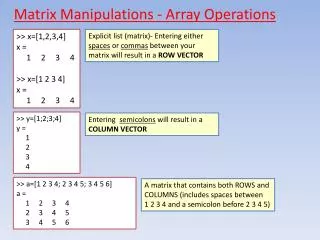
Matrix Manipulations - Array Operations >> x=[1,2,3,4] x = 1 2 3 4 >> x=[1 2 3 4] x = 1 2 3 4 Explicit list (matrix)- Entering either spaces or commas between your matrix will result in a ROW VECTOR >> y=[1;2;3;4] y = 1 2 3 4 Entering semicolons will result in a COLUMN VECTOR >> a=[1 2 3 4; 2 3 4 5; 3 4 5 6] a = 1 2 3 4 2 3 4 5 3 4 5 6 A matrix that contains both ROWS and COLUMNS (includes spaces between 1 2 3 4 and a semicolon before 2 3 4 5)
First Last >> b=1:5 b = 1 2 3 4 5 >> b=2:5 b = 2 3 4 5 >> b=3:8 b = 3 4 5 6 7 8 >> b=[3:8] b = 3 4 5 6 7 8 If you need to create an evenly spaced array, there is a short cut of using a COLON between your first and last value The [square brackets] are optional
Center Number is the increment in the array >> c=0:6 c = 0 1 2 3 4 5 6 >> c=0:1:6 c = 0 1 2 3 4 5 6 >> c=0:2:6 c = 0 2 4 6 >> c=0:3:6 c = 0 3 6 >> a=7:3:19 a = 7 10 13 16 19 >> a=7:3:18 a = 7 10 13 16 An array from 0-6 increasing by increments of 1 (this is the default) An array from 0-6 increasing by increments of 1(center number) An array from 0-6 increasing by increments of 2(center number) An array from 0-6 increasing by increments of 3(center number) Note: The array always begins with the first number and increases by the second (center)until it reaches the thirdnumber. But look what happens if the third number is not an even multiple of “3” – it is NOT included (hmmmm)
If you want MATLAB to calculate the spacing between elements, you may use the linspace command. Specify the INITIAL VALUE, the FINAL VALUE, and how many TOTAL VALUES you want >> d=linspace(1,10,5) d = 1.0000 3.2500 5.5000 7.7500 10.0000 >> d=linspace(1,10,4) d = 1 4 7 10 >> d=linspace(1,10,3) d = 1.0000 5.5000 10.0000 >> d=linspace(1,10,2) d = 1 10 >> d=linspace(2,7,4) d = 2.0000 3.6667 5.3333 7.0000 Five numbers equally spaced between 1 and 10 Four numbers equally spaced between 1 and 10 Three numbers equally spaced between 1 and 10 Two numbers equally spaced between 1 and 10 Four numbers equally spaced between 2 and 7
You can create logarithmically spaced vectors with the logspace command, which also requires three inputs. The first two values are powers of 10 representing the initial and final values in the array. The final value is the number of the elements in the array. Thus: >> e=logspace(1,5,3) e = 10 1000 100000 >> e=logspace(1,5,2) e = 10 100000 >> e=logspace(1,3,3) e = 10 100 1000 >> e=logspace(1,3,2) e = 10 1000 >> e=logspace(0,6,4) e = 1 100 10000 1000000 1= 10^1, 5= 10^5, 3=three values (initial) (final) (# of elements) 1= 10^1, 5= 10^5, 2=two values 1= 10^1, 3= 10^3, 3=three values 1= 10^1, 3= 10^3, 2=two values 0= 10^0, 6= 10^6, 4=four values
Matrices can be used in many calculations with scalars. If a=[1 2 3], we can add five to each value in the matrix as follows: >> a=[1 2 3] a = 1 2 3 >> b=a+5 b = 6 7 8 >> c=a+10 c = 11 12 13 (this was just to define the matrix (array) for “a” (added five to each number in the matrix “a”) 1+5 = 6 2+5 = 7 3+5 = 8 (added 10 to each number in the matrix “a”) This works great for addition and subtraction. BUT, things need to be different when we need to multiply and divide by another matrix.
For multiplication and division we need the operator to indicate element-by-element multiplication. The operator is .* (called dot multiplication or array multiplication). (.*) >> a=[1 2 3] a = 1 2 3 >> b=[6 7 8] b = 6 7 8 >> a.*b ans = 6 14 24 >> (this was just to define the matrix (array) for “a” (this was just to define the matrix (array) for “b” To multiply a*b notice the .* between “a” and “b” Look what happens if you enter a*b (results in Error) >> a*b ??? Error using ==> mtimes Inner matrix dimensions must agree. Element 1 of matrix “a” being multiplied by element 1 of matrix “b” (1*6) = 6 Element 2 of matrix “a” being multiplied by element 2 of matrix “b” (2*7) = 14 Element 3 of matrix “a” being multiplied by element 3 of matrix “b” (3*8) = 24
Other mathematical operations with matrixes (notice the . - dot) >> a=[1 2 3] a = 1 2 3 >> a.*4 ans = 4 8 12 >> a.^2 ans = 1 4 9 >> a.^3 ans = 1 8 27 >> a./2 ans = 0.5000 1.0000 1.5000 (this was just to define the matrix (array) for “a” Multiplying by 4 to elements of a (1, 2, 3) by * 4 1*4=4 2*4=8 3*4=12 Squaring all elements of a (1, 2, 3) ^2 1^2=1 2^2=4 3^2=9 Cubing all elements of a (1, 2, 3) ^3 1^3=1 2^3=8 3^3=27 Dividing by 2 to all elements of a (1, 2, 3) /2 1 /2 =0.5 2 /2 =1.0 3 /2 =1.5
Practice Problems >> a=[2.3 5.8 9] a = 2.3000 5.8000 9.0000 >> sin(a) ans = 0.7457 -0.4646 0.4121 Define the matrix a=[2.3 5.8 9] Find the sine of a. Add 3 to every element in a. Define the matrix b=[5.2 3.14 2] Add together each element in matrix a and in matrix b >> a+3 ans = 5.3000 8.8000 12.0000 >> b=[5.2 3.14 2] b = 5.2000 3.1400 2.0000 >> a+b ans = 7.5000 8.9400 11.0000 2.3 + 5.2 = 7.5 5.8 + 3.14 = 8.94 9+2 = 11
Practice Problems >> a.*b ans = 11.9600 18.2120 18.0000 6. Multiply each element in a by the corresponding element in b 7. Square each element in matrix a 8. Create a matrix c of evenly spaced values from 0 to 10, with an increment of 1. 9. Create a matrix d of evenly spaced values from 0 to 10, with an increment of 2. 10. Use the linspace function to create a matrix (f)of six evenly spaced values from 10 to 20. 2.3 * 5.2 = 11.96 5.8 * 3.14 = 18.212 9*2 = 18 >> a.^2 ans = 5.2900 33.6400 81.0000 >> c=[0:1:10] c = 0 1 2 3 4 5 6 7 8 9 10 Center # is the increment >> d=[0:2:10] d = 0 2 4 6 8 10 Center # is the increment >> f=linspace(10,20,6) f = 10 12 14 16 18 20 (INITIAL VALUE (10), FINAL VALUE (20), and how many TOTAL VALUES (6)
The transpose operator (‘ - an apostrophe) changes rows into columns >> c= [2 4 7 9 12] c = 2 4 7 9 12 >> c‘ ans = 2 4 7 9 12 >> c+2 ans = 4 6 9 11 14 >> c'+2 ans = 4 6 9 11 14 (created a new matrix “c”) The result of c‘+2 changes the answer from a row to a column c‘ changes the answer from a row to a column This (‘) transpose operator is useful when making tables
TABLES – and the transpose operator (‘ - an apostrophe) Suppose we needed to create a table which listed the total cost of bringing several students (1-10) to the movie. Each movie ticket costs $6.00. A table can be created as seen below: >> students=[1:10] students = 1 2 3 4 5 6 7 8 9 10 >> cost=students.*6 cost = 6 12 18 24 30 36 42 48 54 60 >> table=[students', cost'] table = 1 6 2 12 3 18 4 24 5 30 6 36 7 42 8 48 9 54 10 60 (a matrix of 1-10 students) (a new matrix which represents the cost for 1, 2, 3… students at a cost of $6 each) Note that the table requires the (‘) transpose operator for both the students’ and costs’
Now suppose we needed to create a table that showed the conversions between miles per hour (mph) and kilometers per hour (kph). The list for mph should be in increments of five starting at 5 mph through 75 mph. To calculate kph we need to use the conversion factor 1 km = 0.621 mi >> mph=5:5:75 mph = 5 10 15 20 25 30 35 40 45 50 55 60 65 70 75 >> kph=mph/.621 kph = Columns 1 through 10 8.0515 16.1031 24.1546 32.2061 40.2576 48.3092 56.3607 64.4122 72.4638 80.5153 Columns 11 through 15 88.5668 96.6184 104.6699 112.7214 120.7729 >> table=[mph', kph'] table = 5.0000 8.0515 10.0000 16.1031 15.0000 24.1546 20.0000 32.2061 25.0000 40.2576 30.0000 48.3092 35.0000 56.3607 40.0000 64.4122 45.0000 72.4638 50.0000 80.5153 55.0000 88.5668 60.0000 96.6184 65.0000 104.6699 70.0000 112.7214 75.0000 120.7729 (from 5 to 75 – counting by five) Using the conversion factor to calculate kilometers per hour (kph) Note that the table requires the (‘) transpose operator for both the mph’ and kph’ Now, if you are ever traveling to Canada (or any other country in the world) you have a handy chart which shows you the conversions between mph and kph. In Europe, the speed limit is usually about 100 kph (or about 62 mph). But on the German Autobahn, there are places that have no speed limit .