Download
1 / 27
270 likes | 322 Vues
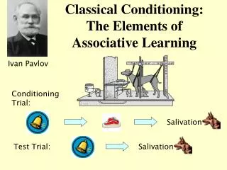
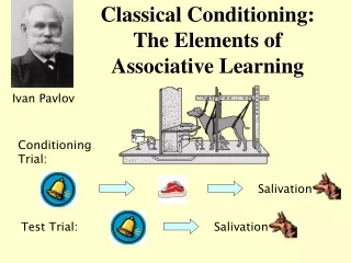
Learn about S-R, R-O, and S-O associations in instrumental conditioning, hierarchical associations, reinforcement theories, stimulus control in behavior, discrimination, generalization, and training effects on behavior control.

E N D
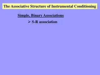
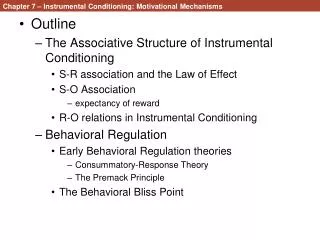
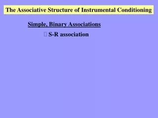
The Associative Structure of Instrumental Conditioning Simple, Binary Associations • S-R association
S-R association T BP food • see more BP during the T than in its absence
The Associative Structure of Instrumental Conditioning Simple, Binary Associations • S-R association • R-O association
R-O association Colwill & Rescorla (1985) Training Devaluation Test R1 O1 O1 LiCL R1 and R2 R2 O2 O2 nothing
The Associative Structure of Instrumental Conditioning Simple, Binary Associations • S-R association • R-O association • S-O association
S-O association Colwill & Rescorla (1988) Sd training Response training Test S1 R3 O1 S1: R3 vs R4 R1 O1 R4 O2 S2: R3 vs R4 S2 R2 O2
The Associative Structure of Instrumental Conditioning Simple, Binary Associations • S-R association • R-O association • S-O association Hierarchical Associations • S – [R – O]
Hierarchical Associations Rescorla (1990) Training Test [R1 O1] S1 S1: R1 vs R2 [R2 O2] S1 S2: R1 vs R2 [R1 O2] S2 [R2 O1] S2 But also, R1 O1 R2 O2
What if we trained: And then gave: R1 – O1 S1 – [R1 – O1] S2 – [R2 – O2] Which S is more informative? Would an increase in responding in the presence of S2 relative to S1 be indicative of a hierarchical association?
Theories of Reinforcement 1. Reinforcement as stimulus presentation Thorndike • a stimulus that is satisfying Hull’s Drive Reduction Theory • any stimulus that satisfies the biological need, Restores homeostasis, and thus reduces the drive state serves as a reinforcer 2. Reinforcement as behavior • The Premack Principle • Behavioral Regulation Approaches
Chapter 8 Stimulus Control of Behavior
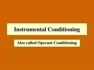
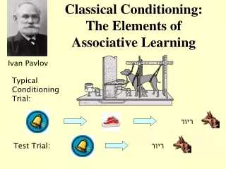
Stimulus Control Classical Conditioning: • Thorndike's original law of effect implied stimulus control. The stimuli (S+/-) present at the time of the reinforced response come to control the response. • The CS (CS+/-) comes to control responding Operant Conditioning:
How do you know that an instrumental response has come under the control of certain stimuli? Reynolds (1961)
Reynolds experiment demonstrated: • Stimulus control • the stimulus control of instrumental behavior • is demonstrated by variations in responding • (differential responding) related to variations • in stimuli • Stimulus discrimination • an organism is said to exhibit stimulus • discrimination if it responds differently to twoor more stimuli If an organism does not discriminate between 2 stimuli, its behavior is not under the control of those cues
Stimulus Generalization and Discrimination To measure the perceived similarity of different stimuli from the training stimulus: • A Generalization Test: • Measure responding when a CS+/- or an S+/- is replaced with test stimuli which are different from (but usually similar to) the original CS or S. • If the stimulus can be changed across a single dimension (e.g., wavelength of light or frequency of sound), then a generalization gradient can be plotted.
Generalization Gradient • obtained by presenting a number of stimuli of different values from the same dimension (e.g., wavelength/color; frequency/pitch) as the CS+/- or S+/- used in training • Generalization is evident to the degree that responding to test stimuli is similar to responding to the training stimulus (flatter gradient). • Discrimination is evident to the degree that responding to test stimuli is different from responding to the training stimulus (more peaked gradient).
The Effects of Training Procedures on Generalization and Discrimination Trained to respond (or not) in presence of CS+ or S+ (or CS- or S-). Then usually tested in extinction with a variety of test stimuli • Nondifferential Training : • S+ always present.
Similar to Figure p. 234 in text Flat gradient More generalization
The Effects of Training Procedures on Generalization and Discrimination • Nondifferential Training : • - S+ always present. • Differential (or Discrimination) Training: - Presence/Absence Training: • * reinforced in presence of S+, not in its absence.
Similar to Figure p. 234 in text Flat gradient More generalization More peaked gradient Less generalization; more discrimination
The Effects of Training Procedures on Generalization and Discrimination • Nondifferential Training : • - S+ always present. • Differential (or Discrimination) Training: - Presence/Absence Training: • * reinforced in presence of S+, not in its absence. • - Intradimensional Training: • * reinforced in presence of S+ (e.g., tone of 1000 cps) and not reinforced in presence of S- (e.g., tone of 950 cps), S+ and S- from the same dimension.
Similar to Figure p. 234 in text Flat gradient Non-Differential More peaked gradient Less generalization; more discrimination Presence/Absence Most peaked gradient Intradimensional Least generalization; most discrimination
Spence’s Theory of Discrimination Learning Following Intradimensional Training: • For the S+ (or CS+), there is an excitatory generalization gradient around it. That is, S+ (or CS+) elicits the most responding; similar stimuli also elicit responding, with the greater the similarity, the greater the tendency to respond. • For the S- (or CS-) there is an inhibitory gradient around it. The most inhibition is produced by S-, but similar stimuli also inhibit responding. The greater the similarity, the greater the tendency to inhibit responding.
Peak Shift: Explained by Spence’s Theory of Discrimination Learning • Peak Shift: • occurs when the peak of responding is shifted away from the original S+ in a direction opposite to that of the S-. • Spence's theory explains the Peak Shift: • There is an excitatory gradient around S+ and an inhibitory gradient around S-. • Observed responding is determined by the sum of the two gradients. • Peak shift occurs because the inhibitory gradient around S- subtracts more from the excitation at S+ and between S+ and S- than it does from stimuli similar to S+ that are further away from S-.