Basic sampling distributions
Basic sampling distributions. Distributions and properties. Sampling Distributions. In modern SPC, we concentrate on the process and use sampling to tell us about the current state of the process, i.e. what is the current state of quality related characteristics of the process.


Basic sampling distributions
E N D
Presentation Transcript
Basic sampling distributions Distributions and properties
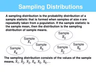
Sampling Distributions • In modern SPC, we concentrate on the process and use sampling to tell us about the current state of the process, i.e. what is the current state of quality related characteristics of the process. • From our random sample, we measure a quality related characteristic(s) and summarize it in a Statistic which is a numerical summary of a sample. • We then relate the Statistical value to a population parameter which is a numerical summary of the population.
Distributions arising in SPC • The distribution of a sample Statistic tells us what we can infer about the current state of the process. • The types of distributions which arise depend on the type of data we collect, qualitative or quantitative. • Qualitative data can only indirectly be given a numerical value since it depends on the presence or absence of an attribute. We can count the number in a sample with that attribute. Example, defective or not. • Quantitative data occurs when the quality related characteristic occurs on a continuous measurement scale. We can take the average value of the characteristic.
Binomial distribution. • Suppose that a process produces items with a fixed proportion of defects, say p. • Suppose items are defective or not independently of each other. • If we take a random sample of size n from a day’s production and count X=number defective out of n, then:
Mean and variance of Binomial • The mean of X, denoted E(X), is given by E(X)=np and the variance of X, denoted Var(X), is given by Var(X)=np(1-p). • One can think of E(X) as the average number of defects in a sample. Note that while the number of defects in any particular sample is an integer, E(X) will not usually be. • The standard deviation of X, denoted σ, is given by the square root of the variance.
Geometric distribution • Often in SPC one waits until a certain event happens such as “how many parts are produced until one is defective” or “how long will we monitor a process until it shows signs that it is unstable”. • If the probability that the event occurs is p, events are independent and X= time until event occurs then
Mean and variance of Geometric distribution • The mean and variance of the geometric distribution are given by • So for example, if we get a signal the process is unstable .01 of the time, then we wait, on average about 100 samples until we get a signal the process is unstable.
Hypergeometric distribution • Suppose items are shipped in lots. A lot has N items in it, of which D are defective. • A sample of size n is taken and X is the number of defectives in the sample. • We wish to evaluate the lot based upon the sample so we need the probability distribution of the number of defects in the sample.
Hypergeometric distribution function • If we sample n items from the lot and count X=number defectives in the sample, then for r=0, 1,…,n:
Facts about Hypergeometric distribution • The mean, E(X)=n(D/N). • Var(X)=n(D/N)((N-D)/N)((N-n)/(N-1)) • If n/N is “small”, say n/N<0.05, then the Hypergeometric distribution is very close to the Binomial distribution.
Poisson distribution • Suppose that we examine a sheet of material and count X=the number of blemishes. Then if X has the Poisson distribution with parameter lambda=λ, and
Discrete vs. continuous distributions • In the previous examples the sampling distributions arose in situations where we observed a process, sampled it, then recorded some property of the members of the sample related to attributes, that is to say qualitative characteristics. • In many, if not most samples, we measure a characteristic of elements of the sample which is on a continuous scale.
Normal distribution (you should all know this) • If we randomly sample an item X from a population whose elements have a normal distribution with mean=µ and variance=σ2, then the density function of X is of the form
Where do these distributions arise in SPC? If we are monitoring a process by sampling from it over time and measuring items in the sample: • If we count the number of defectives in a sample of size n, the distribution is likely Binomial. • If we count the number of blemishes in a continuous area of a certain size, the distribution is likely to be Poisson. • If we measure a continuous characteristic of each item in a sample and average the values, the distribution we use is likely to be Normal.
Distributions continued • If we are using sampling to decide whether or not to accept a lot based upon the number of defects in a sample, we use the Hypergeometric distribution. This occurs late in the course in Acceptance Sampling. • We monitor processes for stability and wait for a signal the process is unstable by monitoring samples over time. The Geometric distribution is used here.