Download
1 / 1
10 likes | 111 Vues
0.4. 0.3. 0.2. 0.1. Cl1 Cl2 Cl3 Non Class. Wind Regimes of Southern California winter S. Conil 1,2 , A. Hall 1 and M. Ghil 1,2

E N D
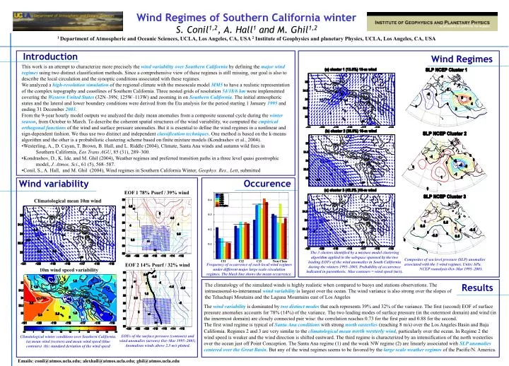
0.4 0.3 0.2 0.1 Cl1 Cl2 Cl3 Non Class Wind Regimes of Southern California winter S. Conil1,2, A. Hall1 and M. Ghil1,2 1 Department of Atmospheric and Oceanic Sciences, UCLA, Los Angeles, CA, USA 2 Institute of Geophysics and planetary Physics, UCLA, Los Angeles, CA, USA Introduction Wind Regimes • This work is an attempt to characterize more precisely the wind variability over Southern California by defining the major wind regimes using two distinct classification methods. Since a comprehensive view of these regimes is still missing, our goal is also to describe the local circulation and the synoptic conditions associated with these regimes. • We analyzed a high-resolution simulation of the regional climate with the mesoscale model MM5 to have a realistic representation of the complex topography and coastlines of Southern California. Three nested grids of resolution 54/18/6 km were implemented covering the Western United States (32N–39N; 125W–113W) and zooming in on Southern California. The initial atmospheric states and the lateral and lower boundary conditions were derived from the Eta analysis for the period starting 1 January 1995 and ending 31 December 2003. • From the 9-year hourly model outputs we analyzed the daily mean anomalies from a composite seasonal cycle during the winter season, from October to March. To describe the coherent spatial structures of the wind variability, we computed the empirical orthogonal functions of the wind and surface pressure anomalies. But it is essential to define the wind regimes in a nonlinear and sign-dependent fashion. We thus use two distinct and independent classification techniques. One method is based on the k-means algorithm and the other is a probabilistic clustering scheme based on finite mixture models (Kondrashov et al., 2004). • Westerling, A., D. Cayan, T. Brown, B. Hall, and L. Riddle (2004), Climate, Santa Ana winds and autumn wild fires in Southern California, Eos Trans AGU, 85 (31), 289–300. • Kondrashov, D., K. Ide, and M. Ghil (2004), Weather regimes and preferred transition paths in a three level quasi geostrophic model, J. Atmos. Sci., 61 (5), 568–587. • Conil, S., A. Hall, and M. Ghil (2004), Wind regimes in Southern California Winter, Geophys. Res., Lett, submitted Wind variability Occurence EOF 1 78% Psurf / 39% wind Climatological mean 10m wind The 3 clusters identified by a mixture model clustering algorithm applied in the subspace spanned by the two leading EOFs of the wind anomalies in South California during the winters 1995–2003. Probability of occurrence indicated in parenthesis. blue contours = wind speed (m/s). Composites of sea level pressure (SLP) anomalies associated with the 3 wind regimes. Units: hPa. NCEP reanalysis Oct–Mar 1995–2003. EOF 2 14% Psurf / 32% wind Frequency of occurrence of each local wind regimes under different major large scale circulation regimes. The black line shows the mean occurrence. 10m wind speed variability The climatology of the simulated winds is highly realistic when compared to buoys and stations observations. The intraseasonal-to-interannual wind variability is largest over the ocean. The wind variance is also strong over the slopes of the Tehachapi Moutains and the Laguna Mountains east of Los Angeles Results The wind variability is dominated by two distinct modes that each represents 39% and 32% of the variance. The first (second) EOF of surface pressure anomalies accounts for 78% (14%) of the variance. The two leading modes of surface pressure (in the outermost domain) and wind (in the innermost domain) are closely connected pair wise: the correlation reaches 0.73 for the first pair and 0.88 for the second. The first wind regime is typical of Santa Ana conditions with strong north easterlies (reaching 8 m/s) over the Los Angeles Basin and Baja California. Regimes 2 and 3 are very similar to the climatological mean north westerly wind, particularly over the ocean. In Regime 2 the wind speed is weaker and the wind direction is shifted eastward. The third regime is characterized by an intensification of the north westerlies over the ocean just off Point Conception. The Santa Ana regime (1) and the weak NW regime (2) are linearly associated with SLP anomaliescentered over the Great Basin. But any of the wind regimes seems to be favored by the large scale weather regimes of the Pacific/N. America. EOFs of the surface pressure (contours) and wind anomalies (arrows) Oct–Mar 1995–2003; Anomalous winds above 2.5 m/s plotted. Climatological winter conditions over Southern California. (a) mean wind (vectors) and mean wind speed (blue contours) (b): standard deviation of the wind speed Emails: conil@atmos.ucla.edu; alexhall@atmos.ucla.edu; ghil@atmos.ucla.edu