Download
1 / 35
350 likes | 564 Vues
Lecture Notes: Econ 203 Introductory Microeconomics Course summary of chapters 1-18 M. Cary Leahey Manhattan College Fall 2012. Chapter 1: The nature of economics; what is economics all about. Allocation of scarce resources Households: decisions to work, save and spend

E N D
Lecture Notes: Econ 203 Introductory MicroeconomicsCourse summary of chapters 1-18M. Cary LeaheyManhattan CollegeFall 2012
Chapter 1: The nature of economics; what is economics all about • Allocation of scarce resources • Households: decisions to work, save and spend • Firms: produce, hire/fire, and distribute those goods • Society: dividing those resources
Chapter 2: economic thinking and practice • Economists explain the world using models with built-in assumptions • Two simple models are circular flow and the PPF • Micro is the study of individual behavior; macro is on the aggregate • Positive (science) versus normative (values) economics
Models: circular flow diagram • Circular flow-visual model of economy • Two types of economic actors: households and firms • Two markets: goods and services and factors of production
Figure 1: The circular-flow diagram Revenue Spending Markets for Goods & Services G & S sold G & S bought Firms Households Factors of production Labor, land, capital Markets for Factors of Production Income Wages, rent, profit 5
Models: Production possibilities frontier (PPF) • The PPF shows the combinations of 2 goods (x, y axis) that can be produced given available resources • Review points along the PPF from Figure 2 • PPF is possible and efficiency • PPF and opportunity cost-shifting resources along the PPF • Slope of PPF is the opportunity cost—the rise over the run
Figure 2: PPF Example E D C B A 7
Chapter 3 Interdependence and gains from trade Interdependence allows everyone to be better off, breaking down the tie between domestic production and domestic consumption Comparative advantage means being able to produce a good at a lower opportunity cost Absolute advantage means being able to produce a good with fewer inputs. Absolute advantage is not needed for comparative advantage. 8
Chapter 4 Supply and demand Competitive (pure/atomistic) market – many buyers and sellers, each of whom has no influence on prices. They are price takers. Supply and demand curves are simplifying tools (models) used to study markets. Demand curve is downward sloping, as price is inversely related to quantity demanded. Supply curve is upward sloping, as prices in positively related to quantity supplied. Prices move along the curve; other factors shift the curves. The intersection of supply and demand determines the equilibrium price. To analyze impacts on markets, see if the example studied shifts supply, demand or both. Examine the relative shifts in the curve and where the new equilibrium plays out and is compared to the old one. 9
Chapter 5: Elasticities Elasticity measures the responsive of Qs and Qd to change in one of its determinants, usually price. Defines as the % change in Qs or Qd / % change in P Unitary elasticity = % change in Q = % change in P Elastic = % change in Q > % change in P Inelastic = % change in Q < % change in P Elasticities tend to rise from the short-run to the long-run Cross price elasticity of demand measures responsiveness of Qd of good 1 to change in price of good 2 Substitutes have a positive elasticity Complements have a negative elasticity 10
Chapter 6: Govt. policies, tax wedges, and incidence Price ceiling is a legal maximum of a price of a good or service. One local example is rent control. If the price is below the equilibrium price, then the price is binding and causes a shortage. A price floor is a legal minimum on the price of a good or service. One example is the minimum wage. If the price floor is above the equilibrium price, it is binding and causes a surplus (unemployment). A minimum wage causes incomes to increase for those who keep their jobs but also causes unemployment among unskilled workers. A tax is a wedge between the price buyers pay and sellers receive, causing equilibrium quantity to fall, regardless on whether it falls on buyers or sellers. The incidence or burden of the tax depends on the elasticities of supply and demand. If supply is more elastic, the incidence or burden falls on the buyers rather than the sellers. And vice versa. Good example is the surprising incidence of a luxury tax on yachts. . 11
Chapter 7: Welfare Another principle fleshed out using welfare economics– market (under certain restrictions) are pretty good at organizing economic activity (efficiency). Distribution can be another story (equity). Modifying these restrictions can invalidate the efficiency outcome. Market failures occur: when one buyer has market power (monopoly) transactions have side effects-externalities (pollution) Buzzwords – invisible hand/laissez faire 12
Chapter 7: Welfare II The height of the D curve reflects the value of the good to buyers—their willingness to pay for it. Consumer surplus is the difference between what buyers are willing to pay for a good and what they actually pay. On the graph, consumer surplus is the area between P and the D curve. The height of the S curve is sellers’ cost of producing the good. Sellers are willing to sell if the price they get is at least as high as their cost. Producer surplus is the difference between what sellers receive for a good and their cost of producing it. On the graph, producer surplus is the area between P and the S curve.
Chapter 7: Welfare III To measure society’s well-being, we use total surplus, the sum of consumer and producer surplus. Efficiency means that total surplus is maximized, that the goods are produced by sellers with lowest cost, and that they are consumed by buyers who most value them. Under perfect competition, the market outcome is efficient. Altering it would reduce total surplus.
Chapter 8: costs of taxation Taxes reduce the welfare of buyers and sellers. This welfare loss usually exceeds the revenue gain. The decline in total surplus (consumer surplus and producer surplus and tax revenue) is called the deadweight loss of the tax. Taxes have deadweight losses because they cause consumers to buy less and seller to sell less, thus shrinking the market. The size of the DWLs depend on the elasticities of supply and demand. Higher elasticities imply higher DWLs. DWLs increases even more than the size of the tax. In one extreme case, revenue may actually fall as taxes become too large. But this rarely happens in real life. 15
The effects of a tax P S PE D Q QE Without a tax, CS = A + B + C PS = D + E + F A Tax revenue = 0 B C Total surplus= CS + PS = A + B + C + D + E + F E D F QT
Chapter 9 international trade Exporting country. A country will export if the world price is above the domestic price without trade. Trade raises the producer surplus, reduces consumer surplus, and raises total surplus. Importing country. A country will import a good is the world price is below the domestic price without trade. Trade lowers the producer surplus but raises consumer surplus and the total surplus. Tariff. A tariff benefits producers and produces revenue for the govt. but the overall economy loses as the gains are less than the losses to consumers. Common arguments for restricting trade include: protecting jobs, defending national security, helping infant industries, preventing unfair competition, and responding to foreign trade restrictions. Only a few (and under restrictive assumptions) have much merit. Free trade is usually the better policy, particularly if the winners can compensate the losers. 17
Summary of the welfare effects from trade PD < PW PD > PW exports imports falls rises rises falls rises rises 0 direction of trade consumer surplus producer surplus total surplus Whether a good is imported or exported, trade creates winners and losers. But the gains exceed the losses.
Chapter 10:externalities Negative externality: market Q larger than socially desirable Q Positive externality: market Q less than socially desirable Q To remedy the problem, internalize the externality Tax goods with negative externalities Subsidize goods with positive externalities. 19
Chapter 11: Public goods Characteristics of goods Excludable-someone can be prevented from using the good Rival-if the consumption of one can reduce the ability of another to consume Private goods are rival and excludable and are the kinds of goods markets work best with Public goods are neither excludable nor rival in consumption This promotes the problem of free riders: consumer do not have to pay, so firms will be less willing to provide those goods. Govts tend to provide public goods, guided by cost benefit analysis to figure ought how much to provide. Common resources are rival in consumption but not excludable, such as grazing land, air/water, and congested roads. The line between private/public goods/common resources is not always clean. People tend to overuse common resources so govts try to limit their use by taxes or regulation. 20
Chapter 12: taxation, equity, and efficiency We introduced a host of new concepts as well as a review of the US tax system The US tax system finds that federal taxes are dominated by income taxes on households while state and local govt taxes are more equally distributed between income, property and sales taxes. Efficiency of the tax system refers to the costs imposed beyond the revenues raised. One measure is the DWL of the distortions. Equity of the tax system refers to fairness which is harder to agree upon than efficiency. The benefits principle refers to those that benefit more pay more in taxes. Ability to pay refers to the ability to handle the burden. The US has a progressive tax system in which higher incomes pay a higher proportion in taxes. Tax incidence can mean that those who bear the tax burden may not ultimately pay the taxes. Policymakers face the tradeoff between goals of efficiency and equity. Notions of horizontal and vertical equity may conflict (example of the marriage tax). 21
Chapter 13: costs of production Costs are both explicit (in cash) or implicit (no cash outlay but an opportunity cost). Both are important to the firm’s decision making Accounting profit is revenue less cash outlays; economic profit is revenue less all (explicit and implicit) costs Production function shows relationship between inputs and output. Marginal production is the increase in output coming from one additional input. Labor is the most common example. Marginal product usually diminishes with insensitivity of use. As output rise the production function becomes flatter (the delta declines) and the total cost curve becomes steeper (delta increases) Variable costs vary with output; fixed costs do not Marginal cost is the increase in total cost from an extra (incremental) unit of production,. The MC curve is usually upward sloping. 22
Chapter 13: costs of production II Average variable cost is variable cost divided by output Average fixed cost is fixed cost divided by output. AFC always falls as output rises. Average total cost (cost per unit or unit cost) is total cost divided by the quantity of output. ATC curve is usually U-shaped. The MC curve intersects the ATC curve at the minimum average total cost MC < ATC, ATC falls as Q rises MC > ATC, ATC rises as Q In the long-run, all costs are variable Economies of scale: ATC falls as Q rises Diseconomies of scale: ATC rises as Q rises Constant returns to scale: ATC remains the same as Q rises 23
EXAMPLE 2: ATC and MC and profit maximization $200 $175 $150 $125 Costs $100 ATC $75 MC $50 $25 $0 0 1 2 3 4 5 6 7 Q 0 When MC < ATC, ATC is falling. When MC > ATC, ATC is rising. The MC curve crosses the ATC curve at the ATC curve’s minimum.
Chapter 14: competitive markets Competitive market is efficient Profit maximization MC = MR Perfect competition P = MR With competitive equilibrium P = MC Since MC is the cost of the last extra unit equal to the value to buyers of that marginal unit, then the competitive equilibrium maximizes total (consumer and producer) surplus Shutdown: a will shut down if P < AVC Exit: a firm will exit if P < ATC With free entry and exit, profits are zero in the long-run, where P = minimum ATC (= MC) 25
SR & LR effects of an increase in demand Market P P S1 MC S2 ATC Profit P2 P2 long-run supply P1 P1 D2 D1 Q Q Q1 Q2 Q3 (market) (firm) 0 A firm begins in long-run eq’m… …but then an increase in demand raises P,… …leading to SR profits for the firm. Over time, profits induce entry, shifting S to the right, reducing P… …driving profits to zero and restoring long-run eq’m. One firm B A C
Chapter 15: monopolies In the real world, pure (natural) monopoly is rare but many firms have market power due to unique products or few competitors Monopoly firm is a sole seller in the market. They arise due to barriers to entry: key resource, govt. granted patent, and economies of scale. Monpolies face a downward sloping demand curve. So price must be lowered on all quantity demanded in order to sell As a result P > MR = MC, leading to a DWL Monopolies earn profits by price discriminating, in which they based pricing decisions to TWP (along the demand curve). Public policy may respond by regulation by creating antitrust laws, breaking up trusts, or by takeovers. All public policies are :issues,” meaning that the best policy may be no policy 27
The monopolist’s profit As with a competitive firm, the monopolist’s profit equals (P – ATC) x Q Costs and Revenue MC ATC ATC D MR Quantity P Q
The welfare cost of monopoly Competitive eq’m: quantity = QC P = MC total surplus is maximized Monopoly eq’m: quantity = QM P > MC deadweight loss Deadweight loss Price MC P P = MC MC D MR QM QC Quantity
Chapter 16: monopolistic competition A MC market has many forms, differentiated products, and free entry/exit. The market is inefficient because of excess capacity and pricing over marginal cost. There may be too much or too little product variety. So a MC market is less desirable than a PC market. MC describes many markets and industries but provides little policy guidance about how to reduce the inherent inefficiencies, since long-run profit in the industry is zero. The goal of product differentiation leads to advertising and branding which may lead to results that are suboptimal. 30
Chapter 17: oligopoly Oligopolies can end up looking like monopolies or like perfect competitors depending on the number of firms and how cooperative the behavior is. Prisoners’ dilemma shows how hard cooperation is, even when it is in all participants best interest. Public policy can employ antitrust laws to increase competition and prevent predatory pricing. The scope of those actions is controversial. Oligopolies maximize profit if they cooperate, form a cartel, and split the monopoly profits. However, self interest leads to an output of greater output and lower price, close to the societal desired outcome. The more firms and the less cooperation leads to a more competitive outcome. 32
Chapter 18: factors of production This is the neoclassical theory of income distribution, in which factor prices are determined by supply and demand and that each factor is paid his value of marginal product. The three factors of production-labor, land and capital. Factor demand is derived from the its supply of output. Competitive firms maximize profits by hiring each factor up to the point where the value of its marginal product equals its rental price. The supply of labor is determined by the work-leisure tradeoff, yielding an upwardly sloping supply curve. The price paid to each factor balances the supply and demand for each factor. In equilibrium, each factor is paid the value of its marginal product. Factors of production are used in conjunction with one another. A change in the quantity of one factor changes the marginal products and earnings of all other factors of production. 33
Equilibrium in the labor market The wage adjusts to balance supply and demand for labor. The wage always equals VMPL. W S W1 D L L1 0
How the rental price of capital Is determined Firms decide how much capital to rent by comparing the price with the value of the marginal product (VMP) of capital. The rental price of capital adjusts to balance supply and demand for capital. P S P D = VMP Q Q 0 The market for capital