Download

1 / 26
260 likes | 500 Vues
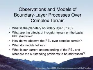
Observations and Models of Boundary-Layer Processes Over Complex Terrain. What is the planetary boundary layer (PBL)? What are the effects of irregular terrain on the basic PBL structure? How do we observe the PBL over complex terrain? What do models tell us?

E N D
Observations and Models of Boundary-Layer Processes Over Complex Terrain • What is the planetary boundary layer (PBL)? • What are the effects of irregular terrain on the basic PBL structure? • How do we observe the PBL over complex terrain? • What do models tell us? • What is our current understanding of the PBL and what are the outstanding problems to be addressed?
Most of our observational and modeling results are relevant to the homogeneous PBL because of its relative simplicity. However, most of the real world land surfaces are far from homogeneous. It is necessary to utilize techniques and instruments that can deal with this extra dimension. Observing the PBL over complex terrain
Techniques for Probing Over Inhomogeneous Terrain • Remote sensing – lidars and radars – can scan both • horizontally and vertically, but have sensitivity and • resolution limitations • Aircraft – fast and mobile, but cannot do long-term • observations • Arrays of instruments – limited by number of sensors • and deployment difficulties
free → troposphere mixed → layer surface → layer
Normalized mixed-layer spectra for the 3 velocity components. The two curves define the envelopes of spectra that fall within the z/zi range indicated. The dashed blue lines indicate contri- butions to the u and v spectra due to mesoscale variability, both from synoptic systems and from surface hetero- geneity.
Map of gully substudy for CASES99 in central Kansas, USA. H refers to 2-d sonic anemometers (at 1 m height) and TH to thermistors (at 0.5 m height).
Shallow Drainage Flows – Mahrt, Vickers, Nakamura, Soler, Sun, Burns, & Lenschow – BLM, 101, 2001. Schematic cross-section of prevailing southerly synoptic flow, northerly surface flow down The gully, and easterly flow likely drainage flow from Flint Hills. Numbers identify the Sonic anemometers on the E-W transect. E is to the right and N into the paper.
9-day composited diurnal variation of the 1-m height wind speed (from 2-d sonic anemometers averaged for 5 minutes For gully stations H1 – H5 (Mahrt et al., BLM, 2001).
Composited diurnal variation of 5-min averaged temperature for the 9.7 m and 0.3 m Levels on the gully tower, and for thermistors on the gully bottom (TH4) and at the Top of the slope (TH9) versus local time (Mahrt et al., BLM, 2001).
Vertical profiles of temperature during the early-evening very stable period with gully Flow (2000 LT) and after mixing (2300 LT) on 26 – 27 October.
Temperature time-height cross- Section and 1-hr averaged wind Vectors for 26-27 October 1999 showing northerly gully flow in the gully bottom before 2130 LT and southerly ambient flow at all stations between 2130 and 0130. reference vector on the left represents 0.25 m/s.
Surface energy balance for 26-27 October. H is sensible heat flux; Rn net radiation, G soil heat flux and Res the imbalance = Rn - H - G
Vector composite (resultant winds) for the 9 most stable nights for the 5 sonic anemometer sites.
Radiation Richardson number provides predictor for local slope (gully) flows:
Two RHI lidar scans from HRDL in CASES-99 illustrating the time de- pendence of waves. (a) at 05:30:49 UTC; (b) at 05:34:24 UTC. Note that the vertical scale is 7.5 times the hori- Zontal scale. Lidar Resolution 30 m. (From Blumen et al., Dynamics of Atmospheres and Oceans, 2001, Fig. 4, p. 197).
Banta, et al., 1990: Doppler lidar observations of the 9 Jan 1989 severe downslope windstorm in Boulder Colorado. 5th AMS Conf. On Mt. Meteor., 23 – 29 June 1990, Boulder, CO, USA.2222
430 m 3060 m 3040 m 3060 m 3040 m
What’s going on with the CO? • Stably-stratified flow going down gully at night (up to ~0630 LT) • At 0630 LT flow starts to reverse and go upslope • During transition (0630 to 0830 LT) highest CO occurs as CO is advected in from nearby forested area and very complicated structure occurs • After upslope is well-established (after 1000 LT) horizontal gradients disappear – CBL is well-established