Download
1 / 51
570 likes | 792 Vues
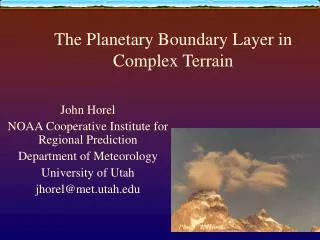
The Planetary Boundary Layer in Complex Terrain. John Horel NOAA Cooperative Institute for Regional Prediction Department of Meteorology University of Utah jhorel@met.utah.edu. Photo: J. Horel. What is CIRP?.

E N D
The Planetary Boundary Layer in Complex Terrain John Horel NOAA Cooperative Institute for Regional Prediction Department of Meteorology University of Utah jhorel@met.utah.edu Photo: J. Horel
What is CIRP? • CIRP: NOAA Cooperative Institute for Regional Prediction at the University of Utah • Mission: Improve weather and climate prediction in regions of complex terrain • People: • Staff: John Horel, Jim Steenburgh, Mike Splitt, Judy Pechmann, Will Cheng, Bryan White, Brian Olsen • Students: Justin Cox, Jay Shafer, Ken Hart, Dave Myrick, Dan Zumpfe, Erik Crossman, Greg West
Barry, R., 1992: Mountain Weather and Climate. Rutledge • Blumen, W., 1990: Atmospheric Processes Over Complex Terrain. American Meteorological Society, Boston, MA. • Clements, C., D. Whiteman, J. Horel, 2003: Cold pool evolution and dynamics in a mountain basin. J. Appl. Meteor., 42, 752-768. • Garratt, J., 1992: The Atmospheric Boundary Layer. Cambridge • Horel, J., M. Splitt, L. Dunn, J. Pechmann, B. White, C. Ciliberti, S. Lazarus, J. Slemmer, D. Zaff, J. Burks, 2002: MesoWest: Cooperative Mesonets in the Western United States. Bull. Amer. Meteor. Soc., 83, 211-226. • Kalnay, E., 2003: Atmospheric Modeling, Data Assimilation and Predictability. Cambridge • Kossmann, M., and A. Sturman, 2003: Pressure-driven channeling effects in bent valleys. J. Appl. Meteor., 42, 151-1158. • Lazarus, S., C. Ciliberti, J. Horel, K. Brewster, 2002: Near-real-time Applications of a Mesoscale Analysis System to Complex Terrain. Wea. Forecasting. 17, 971-1000. • Stull, R. B., 1999: An Introduction to Boundary Layer Meteorology. Kluwer • Whiteman, C. D., 2000: Mountain Meteorology. Oxford • Zhong, S. and J. Fast, 2003: An evaluation of the MM5, RAWMS, and Meso-Eta Models at Subkilometer resolution using VTMX field campaign data in the Salt Lake Valley. Mon. Wea. Rev., 131, 1301-1322. • Notes: Summer School on Mountain Meteorology 2003. http://www.unitn.it/convegni/ssmm.htm References
Outline • Part I- Characteristics/impacts of complex terrain • Part II- Resources for observing surface weather • Part III- Basin boundary layer • Part IV- Mountain-valley and lake breezes
Field Programs • CASES-99 Cooperative Atmosphere-Surface Exchange Study. Kansas. Poulos et al., 2002: BAMS, 83, 555-581. • MAP Mesocale Alpine Program. Alps. Bougeault et al., 2002, BAMS, 82, 433-462. • VTMX Vertical Transport and Mixing Experiment. Salt Lake Valley. Doran et al. 2002, BAMS, 83, 537-551.
www.pnnl.gov/vtmx PBL Issues VTMX Science Plan: • Measurement and modeling of vertical transport and mixing processes in the lowest few kilometers of the atmosphere are problems of fundamental importance for which a fully satisfactory treatment has yet to be achieved • Although a general theoretical understanding of many of the physical phenomena relevant to vertical transport and mixing processes exists, that understanding is incomplete, the representation of various phenomena in models is often poor, and the data needed to test those models are lacking. • The upward and downward movements of air parcels in stable and residual layers of the atmosphere and the interactions between adjacent layers are particularly difficult processes to characterize, and significant difficulties also exist in describing the behavior of the atmosphere during morning and evening transition periods. • Complications due to heterogeneous land surfaces and complex terrain further compromise our ability to treat vertical transport and mixing processes properly.
VTMX Science Questions • What are the fundamental processes that control vertical transport for stable and transition boundary layers? • How can momentum, heat, and moisture fluxes be modeled and predicted in a stratified atmosphere with multiple layers? • What improvements in numerical simulations and forecasts of vertical transport and mixing during stable and transition periods are feasible and how can they be implemented? • What formulations are most appropriate for the description of vertical diffusion in stable air? For example, how rapidly will an elevated layer of pollutants mix towards the ground in a stable pool trapped within a basin, and how can that mixing be modeled? • What is the sensitivity of current local weather forecast and dispersion model predictions to variations in the treatment of vertical diffusivity and turbulence? • What limits our ability to forecast vertical transport in current numerical prediction models? • How do traveling weather systems remove stable stagnant air out of a basin, and under what conditions do these removal mechanisms fail? • What is the nature of the interaction of terrain-induced flows (e.g., drainage winds at night, upslope winds during the day, and waves) with cold air pools in basins, and how do such flows affect the formation and erosion of those pools and the dispersion of pollutants in them?
What are the effects of complex terrain? • Substantial modification of synoptic or meso scale weather systems by dynamical and thermodynamical processes through a considerable depth of the atmosphere • Recurrent generation of distinctive weather conditions, involving dynamically and thermally induced wind systems, cloudiness, and precipitation regimes • Slope and aspect variations on scales of 10-100 m form mosaic of local climates (Barry 1992)
Effects of Complex Terrain Carruthers and Hunt 1990
Billiard ball analogy • “If the earth were greatly reduced in size while maintaining its shape, it would be smoother than a billiard ball”. (Earth radius = 6371 km; Everest = 8.850 km) • Nonetheless, mountains have a large effect on weather. Why is this, if they are so insignificant in size? • Answer: the atmosphere, like the mountains, is also shallow (scale height 8.5 km) so mountains are a significant fraction of atmos depth. • But, this answer underestimates mountain effect for two reasons: • Stability gives the atmosphere a resistance to vertical displacements • The lower atmosphere is rich in water vapor so that slight adiabatic ascent brings the air to saturation. • Example: flow around a 500-m mountain (<< 8.5 km) could include 1) broad horizontal excursions, 2) downslope windstorm on lee side, and 3) torrential orographic rain on windward side. Smith (1979)
Distribution of mountains on the globe (Barry 1992) Total land surface is about 149 million km2. Oceanic islands covering 2 million km2 are not included in the listed areas. Plateau & mountains are both included in the table’s 1st line. Louis (1975)
Energetic Considerations • Since the atmosphere is heated mainly from the ground, cooling effect upon earth’s surface of latent and sensible heat fluxes is nearly double that of radiative fluxes • Since much of the land surface is hilly, thermally driven circulations play important role in global energy balance F. Fiedler. Summer School Trento
Chen, C.-C., D. Durran and G. Hakim(2003) ICAM Surface Wind and Vorticity Around Isolated Mountain: Interaction with Large-scale flow
Potential Temp, Vertical Velocity, and Turbulent Mixing Chen, C.-C., D. Durran and G. Hakim (2003) ICAM
Planetary boundary layer 1 km Height (m) • Energy and mass exchanges near ground • ---interactions among soil science, hydrological cycles • (ground and air), ecosystems, and atmosphere. • Canopy • Terrain • Heterogeneous surfaces • Clouds/fog • Urban environment, air pollution D. Lenschow
Shallow Drainage Flows – Mahrt, Vickers, Nakamura, Soler, Sun, Burns, & Lenschow – BLM, 101, 2001. Schematic cross-section of prevailing southerly synoptic flow, northerly surface flow down The gully, and easterly flow likely drainage flow from Flint Hills. Numbers identify the Sonic anemometers on the E-W transect. E is to the right and N into the paper.
Pollutant Transport in Valleys Nighttime Stable Layer in Valley After Breakup of Nighttime Stable Layer in Valley Savov et al. (2002; JAM)
Daytime vertical mixing processes Jerome Fast
Diurnal mountain wind systems Whiteman (2000)
Mountain-plain circulation, Rocky Mountains US radar profiler network, 1991-1995, Jun-Aug, 500 m gate, max=3.5 m/s Whiteman and Bian (1998)
Mountain-plain circulation in Alps (Vertikator) Emissions within the area of Alpine Pumping are transported into the Alps and mixed convectively to higher levels Boundary of Alpine pumping synoptic conditions modify shape Munich 100 km Zürich Graz Innsbruck Milan Lyon Turin Lugauer et al. (2003)
Vertical cross-section of slope flow (upslope to the right) Mountain venting, anti-slope flow 25 July 2001 CBL Height from Lidar Reuten et al.( 2002) with Steyn
Valley cross sections temperature and wind structure layers at a time midway through the transition Whiteman (2000) Whiteman (1980)
Channeling of synoptic/mesoscale winds Forced Channeling Whiteman (2000) Pressure Driven Channeling
Bent valley with 45° changes in wind direction above valley Kossmann & Sturman (2003)
Dynamic Channeling Kossman and Sturman 2003
High terrain (dark) Flat (tan)Mtn. Valleys (light)A. Reinecke
Normalized surface-layer velocity standard deviations for near neutral conditions in the Adige Valley in the northern Italy alpine region. a is from Panofsky and Dutton, 1984; b the average values from MAP; e/u*2is the normalized turbulence kinetic energy (From de Franceschi, 2002). D. Lenschow
West DEM Grid Points vs. MesoWest Stations Green-West Blue-MesoWest % of Total Valley Flat Mountain
Adding Physiographic Information to MesoWest Land Data Assimilation Systems (LDAS) UMD Vegetation Types Exposure? Forested? Nearby Water? Mountain/Valley? Urban? Slope? Aspect?
MesoWest land characterization * Sites located disproportionately in urban areas and near water resources.
Diurnal Temperature Range A. Reinecke
Diurnal fair weather evolution of bl over a plain Whiteman (2000)
free → troposphere mixed → layer surface → layer D. Lenschow
Diurnal evolution of the convective and stable boundary layers in response to surface heating (sunlight) and cooling. D. Lenschow
Atmospheric structure evolution in valley terrain Whiteman (2000)
Roughness Effects • For well-mixed conditions (near neutral lapse rate) • U2 = u1 ln (z2/zo)/ln(z1/z0) • Roughness length zo=.5 h A/S where h height of obstacle, A- silhouette area, S surface area A/S< .1 • Zo- height where wind approaches 0
Roughness lengths zo for different natural surfaces (from M. de Franceschi, 2002, derived from Wieringa, 1993). zo (m) Landscape Description ________________________________________________________________ 0.0002 Open sea or lake, tidal flat, snow-covered plain, featureless desert, tarmac, concrete with a fetch of several km. 0.005 Featureless land surface without any noticeable obstacles; snow covered or fallow open country 0.03 Level country with low vegetation and isolated obstacles with separations of at least 50 obstacle heights 0.10 Cultivated area with regular cover of low crops; moderately open country with occasional obstacles with separations of at least 20 obstacle heights 0.25 Recently developed “young” landscape with high crops or crops of varying height and scattered obstacles at relative distances of about 15 obstacle heights 0.50 Old cultivated landscape with many rather large obstacle groups separated by open spaces of about 10 obstacle heights; low large vegetation with with small interstices 1.0 Landscape totally and regularly covered with similar sized obstacles with interstices comparable to the obstacle heights; e.g., homogeneous cities
Effects of irregular terrain on PBL structure • Flow over hills (horizontal scale a few km; vertical scale a few 10’s of m up to a fraction of PBL depth) • Flow over heterogeneous surfaces (small-scale variability with discontinuous changes in surface properties) • Inner layer – region where turbulent stresses affect changes in mean flow • Outer layer – height at which shear in upwind profile ceases to be important
Effects of horizontal heterogeneity in surface properties • Changes in surface roughness • Rough to smooth • Smooth to rough • Changes in surface energy fluxes • Sensible heat flux • Latent heat flux • Changes in incoming solar radiation • Cloudiness • Slope
Summary- Impacts of Complex Terrain • Terrain affects atmospheric circulation on local to planetary scales • Terrain induced eddies modify and contribute to the vertical and horizontal exchange of mass, temperature, and moisture in a much stronger manner than turbulent eddies over flat terrain Photo: J. Horel