Two-Way Tables & Statistical Tests
110 likes | 131 Vues
Learn to analyze two-way tables, measure association, infer hypotheses, and calculations of expected cell counts in data sets. Understand Chi-square test, z-test, and Simpson's Paradox. Improve data analysis skills!

Two-Way Tables & Statistical Tests
E N D
Presentation Transcript
The Basics • Two-way table of counts • Organizes data about 2 categorical variables • Row variables run across the table • Column variables run down the table • Row and Column totals provide the marginal distributions of the two variables SEPERATELY
To describe the association between the row and the column variables, use conditional distributions. • To find the conditional distribution of the row variable for one specific value of the column variable, look only at that one column in the table. • Find each entry in the column as a % of the total. • Very useful if the column variable is the explanatory or independent variable.
A three-way table reports the frequencies of each combination of levels of three categorical variables. • A two-way table can be obtained by adding the corresponding entries in these tables. • This is known as aggregating the data.
Bar graphs can also be used to describe an association between 2 categorical variables. • This can be produced in Minitab, under graph, Chart
Simpson’s Paradox • An association or comparison that holds for all of several groups can reverse direction when the data are combine to form a single group. • Fact that observed associations can be misleading when there are lurking variables.
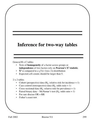
Inference for Two Way Tables • The null hypothesis, Ho, of interest in a two-way table is that there is no association between the row variable and the column variable. • The alternative hypothesis, Ha, is that there is an association. • For an row (r) X column (c) table • Ho states that the c distributions of the row variable are identical. • Ha states that the distributions are not all the same.
Expected Cell Counts • To test the null hypothesis in r x c tables, we compare the observed cell counts with the expected cell counts calculated under the assumption that the null is TRUE. • The test statistic becomes the numerical summary. • Expected cell count =
Chi-Square Statistic • The chi-square statistic is a measure of how much the observed cell counts in a 2-way table diverge from the expected cell counts. • where “observed” is the sample count
The Chi-square Distribution • Again, it is an approximation related to the normal approximation for the binomial distribution • Like the t distributions, the Chi-square distributions form a family described by a single parameter, degrees of freedom. • df = (r – 1) X (c – 1) • See the density curve on page 625. • Table F provides upper critical values.
The Chi-square test and the z test • A comparison of the proportions of “successes” in two populations leads to a 2 X 2 table. • We can compare two populations proportions either by the chi-square test or by the 2-sample z test (proportion test) • These test will always give the exact same result, because the chi-square is equal to the squares of the corresponding N(0,1) critical values. • The advantage of the z test is that it allows us have either a 1 or 2-sided test
