Advances in Tomographic Image Reconstruction Using Content-Adaptive Mesh Modeling
This presentation discusses a novel approach to reconstructing CT images from projection data by employing content-adaptive mesh modeling techniques. The methodology includes feature map extraction, mesh generation, and interpolation to estimate nodal values for image reconstruction. Key algorithms such as Floyd-Steinberg error diffusion and Delaunay triangulation are utilized to enhance the accuracy and efficiency of the reconstruction process. Results and challenges encountered, such as issues with Radon Transform and mesh node positioning, are analyzed, offering insights for future improvements and applications in medical imaging.

Advances in Tomographic Image Reconstruction Using Content-Adaptive Mesh Modeling
E N D
Presentation Transcript
Tomographic Image Reconstruction Using Content-Adaptive Mesh Modeling H. Can Aras November 29-30, 2004 Project Presentation
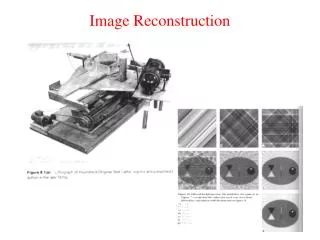
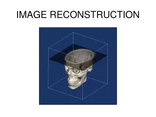
Reconstruction of CT-Images from Projection Data Content-Adaptive Mesh Generation Estimation of Mesh Nodal Values Reconstruction of the Image by Interpolation Problem Approach
Feature Map Extraction • Second derivative used, below is the theoretical basis for this. • M2 : the least upper bound on the second directional derivative of f(x) over T • h : the length of the longest side of T • The formula tells us two things…
Feature Map Extraction (cont.) To achieve a low approximation error of the image: • Small elements in large second derivative regions • Relatively larger elements in relatively small derivative regions
Feature Map Extraction (cont.) • Not practical to calculate directional derivatives • Use max (| fxx |, | fxy |, | fyy |) or the magnitude of the second derivative • Normalization of feature map • Segmentation of heart and background region • Modification of feature map
Placement of Mesh Nodes • Floyd-Steinberg error-diffusion algorithm • Originally designed for digital halftoning • The objective is to use the spatial density of the ink dots to represent the image intensity. • The classical method used varying ink dot sizes.
Placement of Mesh Nodes (cont) • Distribute errors among pixels • Uses the perception characteristics of the human eye • Fast, efficient and produces excellent results (almost)
Connecting Mesh Nodes • Delaunay triangulation • Returns set of triangles such that no data point is contained in any triangle’s circumcircle • Known to yield a well-structured mesh • Avoids producing excessively elongated elements, reducing the error bound
Reconstruction of Image • Pixel value is approximated from the nodal values of its enclosing triangle • Master element • Shape functions
Numerical Comparison • PSNR of FBP result : 47.51 • PSNR of MESH-ML result: 46.77 • compression rate: 5.36 • Note: A higher PSNR does not always correlate well with the perceived image quality (although it provides a measure for relative quality) • A slight change on MESH-ML result gives higher PSNR. • Subtracting only 0.01 from each value of MESH-ML result yields a PSNR of 48.81. Subtracting 0.02 yields 51.05! • The authors may be using another trick for PSNR!
A Comment on Results • The mesh nodal values tend to increase slightly on average after MESH-ML. • Until a number of iterations, the results get better. Behind this limit, results tend to go bad, even worse than FBP (reference) image.
Problems Faced • Radon Transform followed by Inverse Radon Transform yielded an image with negative values because of incomplete set of projections. • I adjusted this image between [0,1] so that the initial values of the mesh nodes are not negative in MESH-ML algorithm.
Problems Faced (cont.) • Delaunay Triangulation is sensitive to the position of the nodes. • Degenerate cases occur frequently when using integers for position coordinates. • I randomly changed the position coordinates with very small differences and used double instead of integer.
Problems Faced (cont.) • The analytical form of the response function is not known. • Hence, I calculated the system matrix by probing the input with an impulse function as offered in the paper. • Specifically, a unit-impulse was applied at each nodal location of the mesh model, and the response at each detector was computed. • This computation is time and memory consuming. • Time problem can be overcome by precalculation. • I used sparse matrix since most of the system matrix is zeros. • The MESH-ML algorithm takes longer than expected.
Plan • Try to make MESH-ML algorithm faster (not the main concern, but can be a bottle-neck for the tests below). • Run MESH-ML with multiple iterations. • Use better reference image in terms of the number of projection angles (5 degrees used between consecutive projections in the experiments). • Use better reference image in terms of the filter used in Fourier domain (Ram-Lak ramp filter used in the experiments). • Test on medical images, which capture different parts of the body.
Thank you for listening… Wish me more luck!